Uncertainty Quantification of Large-Eddy Simulation Results of Riverine Flows: A Field and Numerical Study

Uncertainty Quantification of Large-Eddy Simulation Results of Riverine Flows: A
Field and Numerical Study

K. Flora1, and A. Khosronejad1

1
 Civil Engineering Department, Stony Brook University, Stony Brook, NY 11794
Corresponding author: Ali Khosronejead (ali.khosronejad@stonybrook.edu) Abstract

Abstract
We present large-eddy simulations (LESs) of riverine flow in a study reach in the Sacramento
River, California. The riverbed bathymetry was surveyed in high-resolution using a multibeam
echosounder to construct the computational model of the study area, while the topographies were
defined using aerial photographs taken by an Unmanned Aircraft System (UAS). In a series of
field campaigns, we measured the flow field of the river using the acoustic Doppler current profiler
(ADCP) and estimated using large-scale particle velocimetry of the videos taken during the
operation UAS. We used the measured data of the river flow field to evaluate the accuracy of the
LES-computed hydrodynamics. The propagation of uncertainties in the LES results due to the
variations in the effective roughness height of the riverbed and the inflow discharge of the river
was studied using uncertainty quantification (UQ) analyses. The polynomial chaos expansion
(PCE) method was used to develop a surrogate model, which was randomly sampled sufficiently
by the Monte Carlo Sampling (MCS) method to generate confidence intervals for the LES-
computed velocity field. Also, Sobol indices derived from the PCE coefficients were calculated to
help understand the relative influence of different input parameters on the global uncertainty of
the results. The UQ analysis showed that uncertainties of LES results in the shallow near bank
regions of the river were mainly related to the roughness, while the variation of inflow discharge
leads to uncertainty in the LES results throughout the river, indiscriminately.

1 Introduction
The use of computational fluid dynamic (CFD) models has become more prevalent in hydraulic
modeling of natural systems in recent years due to improvements in high-performance computing
capabilities. Advanced numerical models can provide meaningful insights into the three-
dimensional (3D) flow structures naturally occurring in riverine environments. For example, 3D
computational models can help to understand better the dynamics of the secondary flow at meander
bends, and vortex shedding processes from man-made obstructions such as bridge foundations and
spur dikes (Kang et al., 2020, 2021; Khosronejad, Flora, & Kang, 2020; Khosronejad, Flora,
Zhang, et al., 2020; Khosronejad & Sotiropoulos, 2017). The early use of CFD models for the
study of rivers was limited by computing power to relatively coarse computational meshes and
employed time-averaged Reynolds Averaged Navier-Stokes (RANS) turbulence closure models
(Fischer-Antze et al., 2008; Liang & Fotis, 2005; Liu & García, 2008; Rüther et al., 2010; Wilson
et al., 2003). Recently, more sophisticated, high-fidelity models using detached eddy simulation
(DES) and large eddy simulation (LES) have provided the capability to capture even greater spatial
and temporal details of the flow (Constantinescu et al., 2011; Kara et al., 2015; Khosronejad,
 1

Kozarek, Diplas, et al., 2015; Khosronejad, Kang, et al., 2019). For instance, LES models for full-
scale rivers like the Mississippi River in Minnesota and the Feather River in California have
recently been modeled using LES (Khosronejad, Le et al., 2016; Khosronejad, Flora, & Kang,
2020). Despite these massive improvements in the resolution of the hydrodynamic in rivers, little
attention has been paid to quantifying the results' relative uncertainty. Highly detailed flow
structures may have resulted from considerable uncertainty in modeling parameters and methods,
leading to an excessive level of confidence being placed in modeling results. Furthermore, the
precision offered by highly detailed and impressive results derived from sophisticated numerical
models that were processed by overwhelming computing power may still lead to misleading or,
even worse, incorrect interpretation.
 Uncertainty in numerical modeling arises from many factors, which can be broadly divided
into five primary types: (1) modeling uncertainty, (2) discretization and truncation errors, (3)
convergence errors, and (4) computer round-off errors (Sadrehaghighi, 2020). Some of these
sources of error can be estimated or minimized through increased computational effort, such as
using higher-order numerical schemes, smaller temporal and spatial steps, and specifying reduced
tolerance for reaching convergence (Celik et al., 2008). However, the uncertainty associated with
modeling is often due to model simplifications, limited knowledge of model parameters, boundary
conditions, or accurate calibration data. These types of sources of uncertainty cannot be eliminated
or easily reduced, which makes it necessary to quantifying these types of errors to enable a more
comprehensive understanding of the model results. In particular, hydrodynamic modeling of
natural waterways has many sources of uncertainty. This is due to the spatial nature of the domain,
which is typically large, highly complex, and whose boundaries are frequently changing. In a
typical river, heterogeneity of the channel bed materials, variations in density and types of
vegetation, and complex shapes on the bed, including bedforms and pools, make it impossible to
capture this degree of variation fully and requires many modeling simplifications (Casas et al.,
2010; Flora & Khosronejad, 2021; Lawless & Robert, 2001; Warmink et al., 2011).
 In addition to topography, the inflow boundary conditions could be complicated by
hydrological ambiguity and the error associated with the flow field measurements. Being generated
by rare meteorological events, a sufficiently large number of historical flow rates are often lacking
at the model location, leading to the statistical uncertainty for desired flows of interest.
Additionally, hydrologic uncertainty remains regarding the recorded flow rate data, which are
typically derived from rating curves with inherent errors in both the method and the associated
discharge measurements (Di Baldassarre & Montanari, 2009; Pelletier, 1988). Nowadays,
Acoustic Doppler Current Profilers (ADCPs) are commonly used for estimating discharges in
natural streams because of their relative speed and accuracy. However, ADCPs are known to have
many potential sources of error, including operator error, programming errors, instrument errors,
and extrapolation errors near the bed, water surface, and channel banks (Mueller & Wagner, 2009;
Muste et al., 2010; Muste, Yu, & Spasojevic, 2004; Schmalz et al., 2012). Additionally, when used
for calibration of numerical models, ADCP data can suffer from the practical difficulty of
obtaining enough passes over the same transect line to provide a reliable time-averaged velocity
from the instantaneous data it measures. Nevertheless, with proper operation and post-processing
(Muste, Yu, Pratt, et al., 2004), it is possible to determine accurate average turbulence intensities
and time-averaged velocity field by equally sampling fluctuations higher and lower fluctuations
than the mean value (Fernández-González et al., 2017; Muste, Yu, & Spasojevic, 2004).
Uncertainty in high-fidelity modeling associated with ADCP measurements used for inflow flow
rates was explored in this study.
 2

Another field measurement for riverine models which can be subject to error is inaccurate
or incomplete mapping of the bathymetry of the channel (Casas et al., 2006; Legleiter et al., 2011).
In a case study, Pasternack et al. (Pasternack et al., 2006) estimated that 21 percent of the predicted
depth error in a two-dimensional (2D) model could be attributed to the errors in topographic
resolution. Moreover, in 3D modeling, accurate bathymetry data is critical for determining not
only mean flow characteristics such as depth and mean velocity values but turbulent structures and
secondary velocity components, as well (Keylock et al., 2012; Lane et al., 1999). The uncertainty
associated with delineation of the channel bed surface can result from several sources of
measurement error such as faulty echosounder readings, spatial inaccuracies owing to poor quality
GPS positions, and unaccounted rotations of the boat and sonar transducer. Besides, the low spatial
resolution of the sonar readings, caused by low sampling rates or overly wide spacing between
adjacent vessel passes, can result in missing essential features in the bathymetry and produce
overly simplified channel surfaces. Many of these errors can be reduced or eliminated using (1)
more precise equipment such as augmenting GPS with an inertial navigation unit (INU) for
improved spatial accuracy and (2) a multibeam echosounder (MBES) when possible, instead of a
single-beam echosounder. A comparison of LES results from MBES and single-beam sonar data
showed improved bathymetric resolution reduced near-bed velocities and shear stresses, but
increased the number of turbulent structures in areas with highly irregular topography (Flora &
Khosronejad, 2021).
 Resistance in a channel can be due to many sources, including instream obstacles such as
vegetation and bridge piers, bank irregularities, meander bends, bedforms, and roughness due to
individual grain particles (Recking et al., 2008; Robert, 2003). While the larger features may be
captured in bathymetric/topographic survey data and resolved directly in the discretization of a
high-fidelity model, the surface roughness of the individual grains cannot be practically resolved
when modeling a natural river. Instead, wall models are employed to account for this type of
resistance. Wall models capture different degrees of surface roughness or grain sizes by assigning
an equivalent roughness height value, ! , which is proportional to a characteristic grain size.
Unfortunately, there is no general consensus among researchers for the constant of proportionality
or which specific grain size among the distribution of grain sizes one should use (Camenen et al.,
2006). Chanson (2004) has provided a summary of equivalent roughness heights of several past
researchers regarding flow resistance, which ranged between 1.5 "# by Sumer (1996) in cases of
sheet flow to 3 $# by van Rijn (1984) in bedload transport of experimental and field data. Other
researchers have argued that ! is not only a function of grain size but is a function of the bed load
transport (Camenen & Larson, 2013; Sumer et al., 1996; Yalin, 1992) and the dimensionless
settling velocity rate, as well (Camenen et al., 2006). Regardless, the general lack of consensus
creates uncertainty in what value of ! is appropriate for use in wall models. This study seeks to
investigate how the grain roughness uncertainty impacts the hydrodynamics simulation results of
a field-scale river.
 Hence, the objective of this study is to (1) collect bathymetric and flow measurement data
for a case study in a reach of the Sacramento River in California, (2) conduct high-fidelity large-
eddy simulations (LESs) of the river flow, and (3) quantify the uncertainty in the hydrodynamic
results of the river flow for two input modeling parameters: discharge and the equivalent roughness
height. Specifically, the inflow rate will be varied based on the measurement uncertainty identified
from the ADCP measurements at multiple transects in the river reach. Also, a range of equivalent
roughness height parameters will be used in the wall model to determine how changing the

 3

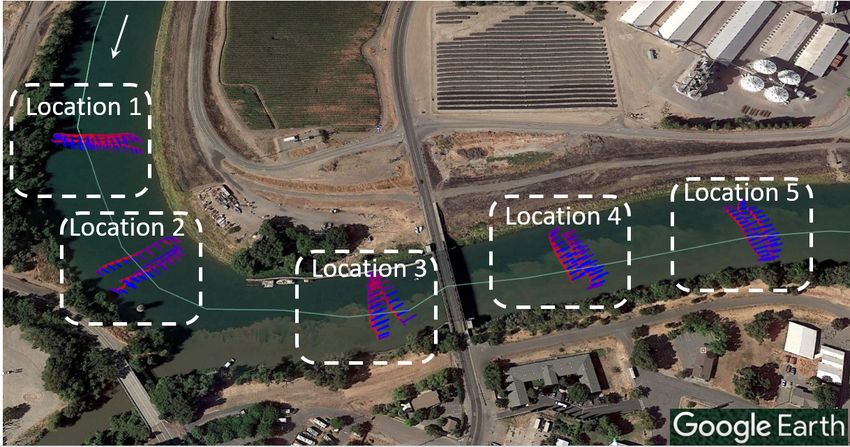
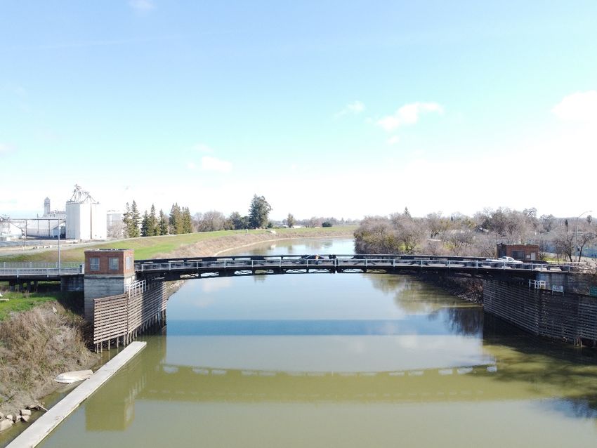
characteristic grain size will alter the flow velocities of this natural river. To quantify the combined
uncertainty of the LES results, polynomial chaos expansion (PCE) and Monte Carlo (MC)
simulations will be used to provide approximate velocities at select transects over a continuous
range of input parameters to generate a 95 percent confidence levels for the computed velocity
fields. Sobol indices, also known as “variance-based sensitivity analysis,” which are used as a form
of global sensitivity analysis, were determined to estimate the relative impact each of these two
parameters has on the hydrodynamics simulation results. Finally, the computed depth-averaged
velocity magnitudes along ADCP transect lines and velocity profiles at select locations were
compared against the measured flow field data.
 The governing equations and the wall model used in the numerical model are introduced
in Section 2. Next, the case study and the field data collection for the river bathymetry and flow
field measurement are discussed in Section 3. Subsequently, the computational details, boundary
conditions, and the range of input parameters for the LES are described in Section 4. Afterward,
the uncertainty quantification procedures are described in Section 5, followed by presenting and
discussing the LES results and UQ analysis of the computed flow field in Section 6. Finally,
conclusions concerning the importance of assessing uncertainty in numerical modeling of natural
rivers are presented in Section 7.

2 Numerical Framework
To simulate instantaneous, 3D, incompressible, turbulent flow for our case study, we use our in-
house, open-source CFD code, the so-called Virtual Flow Simulator (VFS-Geophysics) model.
The successful use of VFS-Geophysics for simulating flow in natural waterways has been well
documented (Giang & Hong, 2019; Kang & Sotiropoulos, 2012; Khosronejad, Le, et al., 2016;
Khosronejad, Kang, et al., 2019; Khosronejad, Flora, & Kang, 2020). For implementing LES in
VFS-Geophysics model, the curvilinear immersed boundary (CURVIB) method described by Ge
and Sotiropoulos (Ge & Sotiropoulos, 2007) is used to resolve the arbitrarily complex geometric
shapes associated with a natural river bathymetry such as channel bedforms, vegetation, bridge
piers, and irregularly shaped banks. In the context of the Immersed Boundary Method (IBM), a
structured background mesh is used for the flow domain. The solid boundaries of objects such as
the channel banks and channel bed are treated as unstructured triangular meshes, which are
superimposed inside the flow domain (Fig. 1). The IBM classifies each node inside the flow
domain as either a solid, fluid, or immersed boundary (IB) node -- as depicted in Fig. 2. As seen,
the nodes shown in the slice in Fig. 2a are designated in Fig 2b as either (1) solid nodes (red region)
which are removed from the computations, (2) fluid nodes (blue region) which reside outside of
the solid boundary where the governing equations for the flow computations are applied, or (3) the
IB nodes (white circles within the gray region) adjacent to the boundary where the velocities are
reconstructed using a wall model.

 4

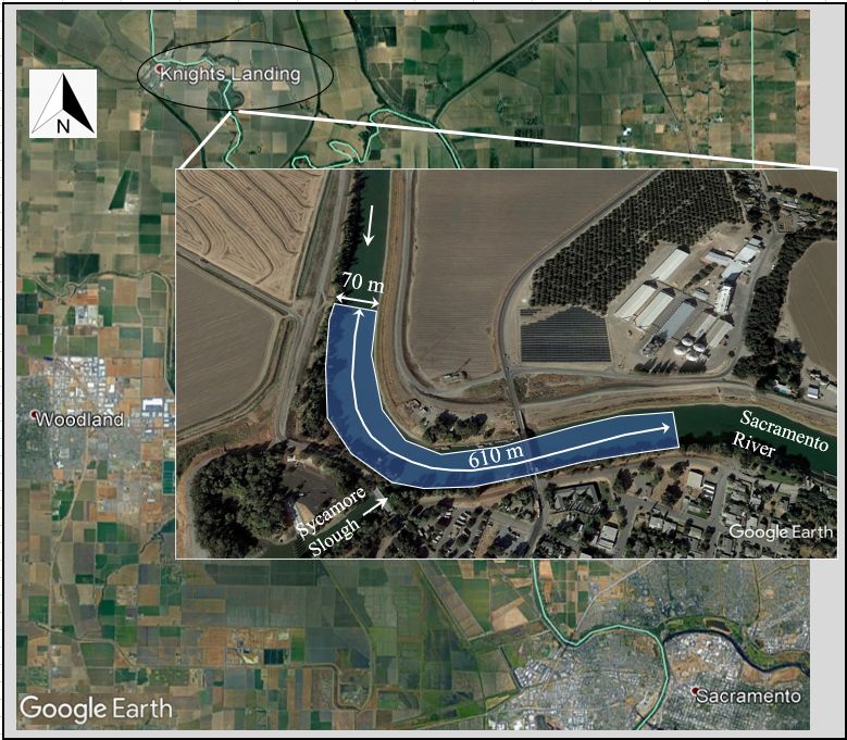
Figure 1. Schematic of the flow domain. The slice outlined in (a) is shown enlarged in (b) with
the white lines representing the structured grid system of the flow domain, and the black triangles
on the bed are the unstructured mesh of the IB.

 5

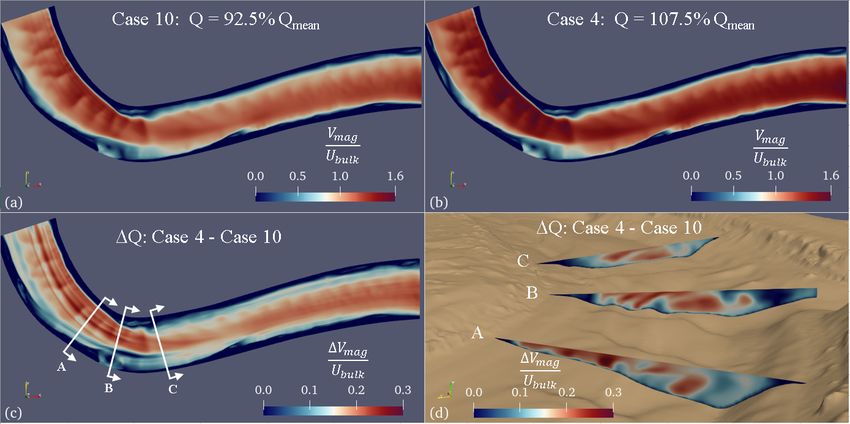
Figure 2. (a) Schematic of a slice taken through channel bed. (b) is an enlarged view of the area
near the riverbed. (b) shows the classification of the background mesh into fluid, solid, and IB
nodes and the location of the nodes adjacent to the wall boundary, where the wall models are
applied.
 In the VFS-Geophysics model, the implementation of LES is fully described by Kang et
al. (Kang et al., 2011) and uses the following algorithm from the Smagorinsky sub-grid scale (SGS)
model (Smagorinsky, 1963);
 '
 %& − ( )) %& = −2 * %& (1)
where µt is the eddy viscosity, and Sij is the large-scale strain-rate tensor. The eddy viscosity, * ,
is defined as:
 * = ! △+ 1 1 (2)
 6

where ! is the Smagorinsky constant, △ is the filter width determined by the grid resolution, and
1 1 is the magnitude of the strain-rate tensor obtained from 1 1 = 22 %& %& .

 In the flow domain, Navier-Stokes equations for incompressible flow are solved in the
hydrodynamic model. The conservation of mass for incompressible flow is expressed as (Ferziger
et al., 2020):
 ,-!
 ,.!
 =0 (3)

where & represents the spatially-filtered velocity components and the conservation of momentum
reads as (Khosronejad & Sotiropoulos, 2014):
 ,-" ,- ' ,0
 ,*
 + & ,.", = − / ,. + ∇+ % + % (4)
 ! "

where ρ is the density of water, P is the pressure, ν is the kinematic viscosity of water, and g is the
gravitational body force.
 A wall model is used to solve indirectly for the velocity at the first grid point off the solid
boundaries (Fig. 2b) for cases when the viscous sublayer itself cannot be resolved directly, such
as in a large flow domain like a natural river and where the individual grains are too small to be
resolved. The wall modeling approach assumes that the first grid points off the wall reside within
the log layer and reads as follows (Khosronejad et al., 2011):
 -
 1 1 ≤ 11.53
 =9' (5)
 -∗ ( 1 ) 1 > 11.53
 2

 5
where is the local velocity magnitude at the node located a distance, , from the wall, ∗ = 2/
is the shear velocity (Wilcox, 1993), is von Karaman’s constant (≈ 0.41), and 1 is the distance
 6-
of the first node off the wall in wall unit (= 7 ∗ ), and E is the roughness parameter, defined as
follows:
 = [Κ( − Δ )] (6)
where
 0 !1 < 2.25
 ⎧ ' 1 1
 Δ = R − 8.5 + 2 ( ! )T [0.4258( ( ! ) − 0.811)] 2.25 < !1 < 90
 ⎨ ' 1
 ⎩ − 8.5 + 2 ( ! ) !1 ≥ 90
 (7)
 ) -
where B is a constant (=5.2) and !1 is the roughness Reynolds number, %8 ∗ , where ! is the
equivalent roughness height. The three cases for Δ in Eqn. 7 represent different effects on the
flow caused by how far above the channel boundary the roughness elements extend, relative to the
viscous sublayer, 9 , where viscous forces dominate. When !1 < 2.25, the roughness elements
are entirely within 9 , where the turbulence generated by roughness elements themselves are fully
dampened out by the viscous forces and do not contribute to the overall channel resistance, which

 7

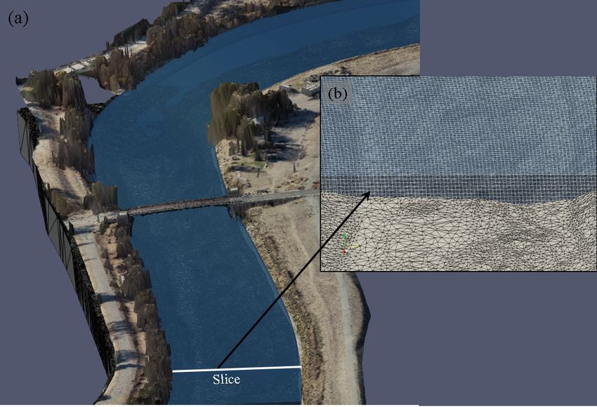
is referred to as hydraulically smooth flow. However, in natural rivers, this condition typically
does not exist since roughness elements generally extend beyond ~5 9 (Robert, 2003). For this
study, ! will be varied to observe how changes in the equivalent roughness height in the wall
model influence the hydrodynamics of the river.

3 Case Study: Sacramento River at Knights Landing

3.1 Site Description
The Sacramento River is a major river in Northern California with headwaters in the Klamath
Mountains which flows over 700 km into the San Francisco Bay-Delta. Approximately 50 km
upstream from the City of Sacramento, the Sacramento River makes a sharp bend -- as it passes
through the town of Knights Landing, CA, which is the site for this case study (Fig. 3). The reach
of interest for our simulations is approximately 610 m long, with a two-lane highway bridge on
Route 113 crossing the river just downstream from the meander bend. The bridge has piers at each
bank protected by timber fenders causing only a minor contraction of flow at the crossing (Fig. 4).
The river in this location is confined by levees on each bank and has an average channel top width
of about 70 m during our field data collection stage. During our field investigation, the mean flow
depth in the channel was about 3.3 m with a deep section approximately 8.5 m deep along the outer
bank located at the channel bend. A side tributary, called Sycamore Slough, enters the Sacramento
River along the right bank near the midlength of the study area. Irrigation water flows into the
slough through a gate located about 400 m upstream from the confluence on Sycamore Slough;
however, this inflow is considered an insignificant addition to the main channel flow in the
Sacramento River.

 8

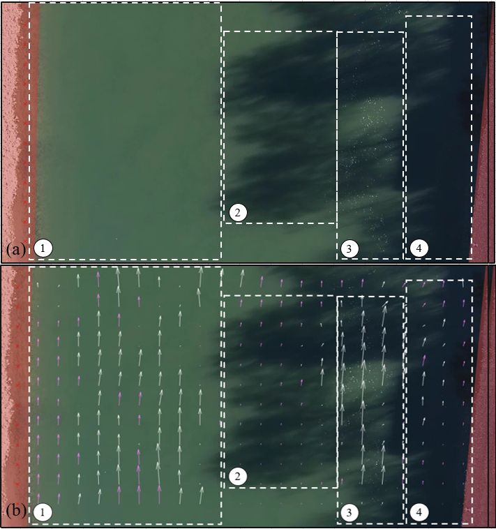
Figure 3. Site map of the study area in the Sacramento River in Knights Landing, California. Flow
is from the North to the East.). (Earth data © 2020 Google.)

 9

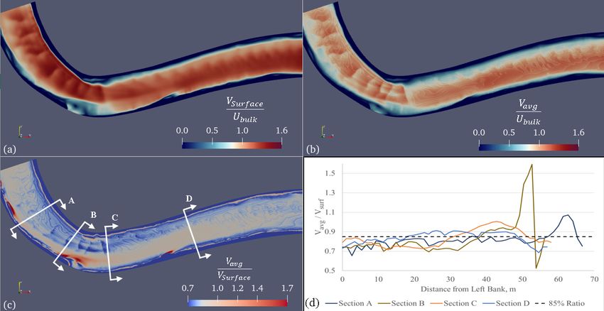
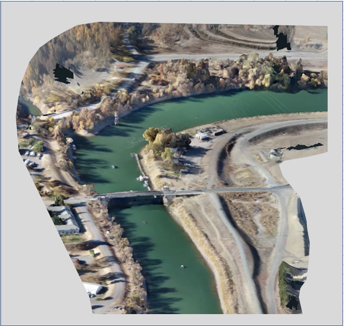
Figure 4. Looking downstream at the Highway 113 bridge crossing over the Sacramento River at
Knights Landing, showing piers protected by timber fenders along each bank.

3.2 Field Measurements
In December 2020, we collected three types of field data: (1) Aerial photogrammetry and video
imagery, (2) ADCP flow field, and (3) bathymetric survey. Herein, the measurement methodology,
equipment used, and the results of each type of data collection are described briefly below. Videos
and images were taken at the site using a DJI Phantom 4 unmanned aircraft system (UAS). Almost
700 4K still photos were taken from an altitude of about 60 m and used to generate topographic
data. This imaging technique is based on the Structure from Motion (SfM) (Fonstad et al., 2013)
methodology, which uses open-source software of OpenDroneMap (Drone Mapping Software -
OpenDroneMap, n.d.). The elevation data above the water surface (Fig. 5) was tied into the 30
ground control points surveyed using a Trimble GeoExplorer 7x GPS unit. This unit allows for
augmenting the bathymetric survey data to generate a complete digital map of the river within the
study reach.

 10

Figure 5. Textured model showing the measured above water topographic data, derived from
aerial photography using SfM for Sacramento River at Knights Landing. Flow is from the top right
to the bottom.

 During the same day, over 20 aerial movies were taken from the field site using the same
DJI Phantom 4 UAS. These animations were used to produce still images, which were then
processed using Large-Scale Particle Image Velocimetry (LSPIV) to obtain the water surface
velocity field of the river. LSPIV was first used by Fujita (1997) to monitor a flood event in Japan
in 1993. Since then, others have successfully employed this method to estimate the water surface
velocity field and turbulence of riverine environments (Fujita et al., 1998; Jin & Liao, 2019; Lewis
& Rhoads, 2015; Sutarto, 2015). LSPIV is an extension of Particle Image Velocimetry (PIV),
commonly used in laboratories where water is seeded with particles and tracked with high-speed
cameras to study flow dynamics in flumes. With LSPIV, naturally or artificial seeded particles
floating on the water surface are similarly tracked over multiple video frames to estimate the
surface velocity magnitude and the direction of the flow. Herein, the videos were shot normal to
the water surface from a stationary UAS for between 30 and 60 seconds and included at least two
control targets with measured coordinates within the field of view. The control targets enable the
scaling of the measurements during the post-processing of the data. The water surface flow
characteristics were analyzed for the most promising videos based on the quantity of seeding using
 11

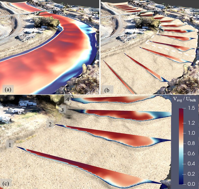
open source software, i.e., RIVeR (Patalano et al., 2017) using only natural seeding consisting
primarily of bubbles and small vegetal debris on the water surface. This software is a graphical
user interface for the MATLAB tool PIVlab designed specifically for LSPIV processing. As seen
in Fig. 6, the seeding and lighting on the water surface varied significantly and strongly influenced
the quality of the results. In Fig. 6(b), Regions 2 and 4 have minimal seeding and poor lighting
conditions. Therefore, the LSPIV processing could not effectively resolve the velocity directly --
requiring the program to extensively interpolate these regions from the resolved velocities in
Regions 1 and 3. Despite minimal seeding, Region 1 still provided reasonable velocity data, which
compared favorably with the other velocity measurements (see Section 6). However, the excessive
uncertainty in the LSPIV velocities proved too great to provide useful flow field data for this study.
The computed depth-averaged results taken as 85 percent of the surface velocities are presented in
Section 6.
 On December 15, 2020, ADCP streamflow measurements were collected using a Teledyne
RD Workhorse Rio Grande® 1200 kHz ADCP and their WinRiver® II data acquisition software.
Spatial data for the survey was obtained using the Advanced Navigation Spatial Dual® Inertial
Navigation Unit (INU). Based on the measured stage from LSPIV data collection of the previous
week, the stage of the river was nearly identical. In total, 17 ADCP transects were made for the
Sacramento River at 5 locations, with three locations being upstream from the highway bridge and
two locations downstream -- see Fig. 7. Flow rates from each transect are shown in Table 1, with
an average flow rate of 130.5 m3/s with a standard deviation of 4.7 m3/s. Variability in the
measurements could be primarily attributed to operator error and a minor inflow from the
Sycamore Slough stream that was measured to be equal to 5.3 m3/s. Each of the five transect
locations was post-processed using the Velocity Mapping Toolbox (VMT) software available from
the USGS (Parsons et al., 2013). Using VMT, multiple transects at each location were combined
to provide a single set of velocity values along a spatially-averaged cross-section to provide a more
time-averaged depiction of the flow than the instantaneous velocities measured during each
transect (Fig. 8). The velocity values were also depth-averaged and used for comparison with the
LES simulations.

 12

Figure 6. (a) An aerial image of the water surface immediately downstream from the highway
bridge. Region 1 has bright sunlight but negligible seeding. Regions 2 and 4 are in the shadows
with poor lighting and minimal seeding. Region 3 has mixed lighting and substantial seeding. (b)
The white arrows are the computed velocity vectors, while the pink arrows are velocity vectors
based on the interpolation.

 13

Figure 7. Locations of the ADCP measurements. The individual transects demonstrating the
depth-averaged flow velocities are presented in blue.

Figure 8. Data post-processing using VMT software. (a) Individual transect lines (blue) and
smoothed averaged transect line (black) for Location 4. (b) depth-averaged velocities along the
smoothed transect line.

 On the same date as the ADCP measurements, a bathymetric survey of the channel bed
was made using a Picotech PICOMB-120 MBES, which operated at 25 pulses per second. The
PICOMB-120 has a 120-degree swath angle projecting 256 beams equally spaced at 0.47 degrees.
Overlapping passes of the operating boat were used to measure the detailed bed bathymetry of the
river. The boat movements and locations were measured using the Advanced Navigation Spatial
Dual INU and post-processed for improved coordinates using Advanced Navigation’s
 14

KinematicaTM algorithms. The heading for the INU was provided using 2 Trimble Zephyr 2
antennas. Over 26 million bathymetric data points were collected and, subsequently, post-
processed using the BeamworXTM Hydrographic Suite of software – see Fig. 9. As clearly seen,
the survey data captured large bedforms that are 1 to 1.5 m high and present throughout the reach.
Also, scour regions that are approximately 4 m deep can be seen along the outer bank of the
meander bend, while about 2 m deep scour regions were detected near the bridge crossing. As
shown in the deeper parts of the river (in blue), the thalweg of the river switches sides by crossing
over from the right bank at the bridge crossing to the left bank near the downstream end of the
study reach. This shift in thalweg is typical of a meandering river and influences the bathymetry
and hydrodynamics, as will be seen in the LES results presented in Section 6.

Figure 9. Bathymetric survey data for the Sacramento River at Knights Landing. Color maps show
the relative bed elevation of the river in meters.

 15

Table 1. Summary of ADCP Measurements. Locations are shown on Fig. 7.

 Location Transect (m3/s)
 1 131.9
 2 122.4
 1
 3 128.5
 4 130.7
 5 124.5
 2 6 124.0
 7 122.9
 8 133.9
 3 9 129.9
 10 136.8
 11 132.8
 12 136.6
 4
 13 134.5
 14 136.3
 15 130.6
 5 16 132.6
 17 130.4

4 Computational Details
The LES of the river flow in the study area was carried out for a mean-flow depth of 3.3 m and
mean-flow rate of 0.565 m3/s, which result in the Reynolds and Froude numbers of 1.86 × 10:
and 0.11, respectively. The flow domain was discretized using a uniform grid node spacing in all
directions equivalent to ~ 0.6 m. For this spacing, 201, 1201, and 21 nodes were placed in the
spanwise, streamwise, and vertical directions, respectively, to create a flow domain with
approximately 5 million computational grid nodes. About half of these nodes were classified as
solid nodes and banked out of the computations. The timestep for all simulations was equivalent
to 0.07s. Typical values for 1 were greater than 1000. Given the Reynolds number of the river
flow in this study, the employed grid resolution is understandingly too coarse to capture the viscous
sublayer of the turbulent flow. However, since in such large-scale riverine flows, large bathymetry
features and other wall-mounted structures are responsible for producing slowly evolving but very
energetic coherent structures, which are responsible for producing most of the turbulence, we have
been able to successfully resolve such flows using wall models (Flora et al., 2021; Khosronejad et
al., 2011, 2012, 2013; Khosronejad, Diplas, Angelidis, et al., 2020; Khosronejad, Flora, & Kang,
2020; Khosronejad, Kozarek, Palmsten, et al., 2015). That is without needing to resolve the details
of the near wall flow, provided that one uses grids fine enough to capture key geometrical features
and resolve the slowly coherent flow structures they induce. This has been the basic premise for
the success of LES linked with the immersed boundary method developed for and introduced in
 16

simulations of river hydrodynamics and morphodynamics (Khosronejad et al., 2013; Khosronejad,
Flora, & Kang, 2020; Khosronejad, Flora, Zhang, et al., 2020; Khosronejad, Le, et al., 2016).
 Based on the field observations of the water surface elevation during the bathymetric
survey, there was minimal variation in the water surface throughout the reach. The water slope of
the river was highly mild (0.005percent). For this reason (Khosronejad, Ghazian Arabi, et al.,
2019), we employed a flat rigid-lid assumption at the free surface to facilitate the computations of
the LESs using the location of the free surface obtained from the measured water surface elevation.
The no-slip boundary condition was prescribed at the wall boundaries and bridge piers. A range of
flow rates for the Sacramento River was assigned at the inlet, as discussed in Section 6. Before
conducting the LESs of the study reach, a short and straight reach with uniform channel geometry
derived from the inlet cross-section of the study reach. This short channel was used to develop
turbulent inlet boundary conditions at the inflow boundary of the study reach. Separate precursor
runs were completed for each discharge used in this study. For each flow rate, when the precursor
simulation reached a fully developed, turbulent flow state, the instantaneous velocity field at the
outlet was stored for later use in the LESs of the study reach. No additional flow was assumed to
enter the flow domain at the confluence with Sycamore Slough.

5 Uncertainty in model parameters
The hydrodynamic results of our LESs are presumed to be highly dependent on two crucial input
parameters: (1) the inflow discharge and (2) the equivalent roughness height. As shown in Table
1, in the study reach, several different flow rates were measured using the ADCP. Using the mean
value of 130.5 m3/s would be a logical choice for inflow discharge. However, one needs to
determine how much uncertainty this mean discharge value will introduce in the LES results? To
quantify this uncertainty, a range of nine different flow rates representing flow rates from 10
percent less than the mean discharge to 10 percent greater than the mean value was simulated. In
addition, the equivalent roughness height, ! , used in the wall model (Eqn. 7) could impact the
computed velocity profiles within the river and possibly redistribute the velocities laterally, as
well. As stated earlier, there is a lack of consensus among researchers for how to define ! . For
this study, several values were used to represent a wide range of potential values for ! .
Specifically, values for the equivalent roughness height ranging between 1.5 "# < ! < 3 $#
were utilized based on the disparity of values and relationships related to ! in literature (Camenen
et al., 2006; Chanson, 2004; Ferguson, 2007; Hey, 1979; Sumer et al., 1996; van Rijn, 1984).
Furthermore, it was assumed that the uncertainty associated with ! is uniformly distributed. The
USGS sampled bed material from the river on November 1, 1977, at the USGS Gage No. 11391000
(USGS 11391000 SACRAMENTO R A KNIGHTS LANDING CA Water Quality Data, n.d.). Based
on three representative sediment samples presented in Fig. 10, "# = 7.0 and $# = 21.6 
making the equivalent roughness height to range between 10 mm and 65 mm. Therefore, for this
study, values of ! equal to 10, 14, 20, 40 and 60 mm were used in the LESs. Due to the
computational cost for running each LES, only 11 cases combining different discharges and
equivalent roughness heights were run (see Table 2). To augment the “gaps” for other
combinations of these two parameters, a PCE was used to estimate the flow field results of all
possible combinations of parameter values for the inflow rate and equivalent roughness height.

 17

Figure 10. Cumulative size distribution for sediment samples of the Sacramento River at Knights
Landing obtained from USGS Gage 11391000. In the insert table, d is the percent finer of the
particle size in mm.

Table 2. Summary of LES scenarios. ! is the equivalent roughness height, !1 is the roughness
Reynolds number, is dimensional flow rate, and the last column shows the percentage of flow
relative to the mean flow rate (130.5 m3/s).

 Case Mean 
 '
 Percent of Mean 
 Number (mm) (m3/s)
 1 10 150 130.5 100
 2 14 210 130.5 100
 3 20 300 130.5 100
 4 20 300 140.3 107.5
 5 40 600 130.5 100
 6 60 900 130.5 100
 7 60 900 120.7 92.5
 8 40 600 137.0 105
 9 40 600 124.0 95
 10 20 300 120.7 92.5
 11 60 900 140.3 107.5

 The PCE is a general methodology that can be used in uncertainty quantification
evaluations, representing the functional relationship between input parameters and the resulting
output rather than only the statistical correlation between the parameter inputs and hydrodynamic
outputs (Adams et al., 2020). Herein, non-intrusive PCE simulations are used as black boxes, and
the calculation of the PCE coefficients for flow velocities is based on the set of LES cases (Eldred,
2009). Once the correct polynomial coefficients are determined, the PCE can approximate finite-

 18

dimensional series expansions of the flow velocities for any input variables. The chaos expansion
for Response R can be approximated as (Eldred, 2009):
 ≅ ∑0&;# & & ( ) (8)
where & is a deterministic coefficient, % is the ith multidimensional orthogonal polynomial, and
 is a vector of standardized random variables. Herein, the Askey family of orthogonal
polynomials are employed for the PCE evaluation. More specifically, since the probability
distributions for the inflow and ! are assumed to be uniformly distributed, the Legendre
orthogonal polynomials are used for the PCE(Narayan & Xiu, 2012).
 To assess the relative sensitivity caused by different variables in the uncertainty of the
hydrodynamics results, the coefficients in PCEs can be analyzed using variance-based
decomposition to extract values known as “Sobol” indices (Sudret, 2008). This analysis identifies
the fraction that either individual variables or a specific combination of variables contribute to the
total uncertainty in the response, Y. This effect is known as the main effect sensitivity index, and
for a single variable, % , is represented by the Sobol Index value, % , which is defined as (Eldred et
al., 1999):
 ( ?@A B % CD
 % = "
 (F)
 (9)

where ." [ ( | % )] represents the variance of the conditional expectation of for a given %
and ( ) is the total variance.
 Once the PCE is evaluated, the full range of inflow rates and equivalent roughness heights
can be explored using the surrogate model by the MC sampling. The MC sampling repeatedly
selects random values of the two parameters and evaluates the corresponding velocities from the
PCE to define the confidence intervals from the statistical variance in the PCE responses. This
process is repeated for each location in the study reach where confidence intervals are desired.
Herein, we evaluate the depth-averaged velocities along 4 of the ADCP locations and at four
vertical profiles, where ADCP measurements were taken. The Design Analysis Kit for
Optimization and Terascale Applications (Dakota) software developed by Sandia National
Laboratory was used to conduct the UQ analysis. Based on the 11 LES cases, Dakota first
determined the PCE coefficients and Sobol indices for the points of interest in the study reach and
then randomly sampled 10,000 combinations of parameter inputs using MC sampling to define 95
percent confidence intervals. Fig. 11 shows the workflow for the UQ analysis.

 19

Figure 11. The flowchart illustrates the process of UQ analysis.

6 Results
Each of the 11 LES Cases listed in Table 2 ran until flow was well established through the reach,
as shown in Fig. 12. This figure shows a large flow separation region occurring along the outer
bend of the river near the confluence with Sycamore Slough. A smaller separation zone is also
noted at the inner bend. Upstream of the bend, flow is relatively uniform, showing only velocity
fluctuations corresponding to the bedforms on the left side of the channel. Due to the meander
bend, however, the flow becomes noticeably less streamlined and exhibits continuous large-scale
turbulence. After the kinetic energy of the flow stabilized, time-averaged results were computed
until the mean statistics converged. Like the instantaneous flow, the small fluctuations in the time-
averaged velocity magnitudes on the water surface reflect the presence of the channel bedforms
throughout the channel and the flow separation along the right bank (Fig. 13 (a)). As seen in Fig.
13 (c), the sharp meander bend leads to large-scale redistribution of the velocity core in the water
column. The strong secondary flow at the bend produces non-typical velocity profiles in vertical,
which can be clearly seen in cross-section 3 of Fig. 13(c). The velocity magnitude at the water
surface elevation is significantly lower than that of mid-depth near the outer bank. Trying to
measure the discharge in this area will likely create inaccurate readings. For instance, if an ADCP
is used, the flow near the water surface cannot be measured directly and is estimated using a
logarithmic profile assumption which is not valid at this location. Similarly, when processing
LSPIV data, the velocities at the water surface are typically reduced to estimate the depth-averaged
value for use in the discharge calculation. As shown, reducing the surface velocity at this location
would be inappropriate based on the computed results.
 Due to the uncertainty in the inflow discharge, several LESs were conducted using identical
equivalent roughness heights while varying only the flow discharge to assess the effect of flow
discharge alone on the computed hydrodynamics. For instance, both Cases 4 and 10 simulated the
flow field using ! = 20 mm but varied the inflow discharge from 140.3 m3/s to 120.7 m3/s that
 20

are 107.5 percent and 92.5 percent of the mean flow, respectively. The time-averaged surface
velocity magnitudes for these two cases are shown in Fig. 14(a) and (b). As expected, the higher
flow rate in Case 4 shows noticeably higher velocity magnitudes at the water surface. However,
when comparing the difference in velocity magnitudes in Fig. 14(c), the increase in velocity
magnitude at the water surface scales nonuniformly concerning the 15 percent difference in
discharges. Upstream of the bend along the inner bend of the river in the shallower parts of the
river, flow velocity magnitudes increase by roughly 30 percent, whereas, along the outer bend, the
velocity magnitudes increase by less than 10 percent. Even more surprisingly, the velocity field
throughout the flow depth scales nonuniformly with the increased flow rate but shows highly
variable increases throughout the study reach (Fig. 14 (d)). We argue that this could be attributed
to the complex secondary flows and nonuniformity of bed bathymetry. The former is known to
cause the lateral movement of the high-velocity core (Kang et al., 2011; Kang & Sotiropoulos,
2012), while the latter is known to produce heterogeneous turbulent flow structures in the water
column (Khosronejad, Hansen, et al., 2016; Le et al., 2019).
 Like the variability in velocity field throughout the river caused by changing the discharge,
LES cases were also computed using different equivalent roughness heights while maintaining the
same flow rate at the inlet. Fig. 15 shows the results from Case 1 and Case 6, which used ! values
of 10 mm and 60 mm, respectively. As seen in Fig. 15 (a) and (b), the velocity magnitudes at the
water surface appear to be quite similar; however, considering the difference in the two surface
velocity magnitudes, one can see that increasing the bed roughness results in a decrease in the
velocity magnitude ranging from 5 to 15 percent along the left bank (see Fig. 15(c)). Conversely,
downstream from the bend along the right bank, increasing the bed roughness leads to an increase
in surface velocities by 5 to 15 percent. Within the bend itself, these effects are even more evident,
causing the same velocity changes to be even more significant. As seen in Fig. 15 (d) at the three
cross-sections in different parts of the bend, the degree and location of the velocity magnitude
changes are nuanced, with varying changes being induced by the roughness seen in other velocity
structures in the cross-sections.
 Typically, the velocity profile of a river flow follows a logarithmic or parabolic profile
(Robert, 2003). Accordingly, the depth-averaged velocity magnitude is often approximated to be
about 85 percent of the surface velocity magnitude (Buchanan et al., 1976). The surface velocity
magnitude and depth-averaged velocity magnitudes are compared for Case 3 to investigate the 85
percent approximation using our simulation results in the study reach of the Sacramento River.
This case corresponds to the inflow rate of 130.5 m3/s and the equivalent roughness height of ! =
20 mm. As seen in Fig. 16 (a) and (b), as expected, the velocity magnitude is generally lower for
the depth-averaged values. Closer examination of the percentage of the depth-averaged velocity
magnitude relative to the surface velocity magnitude in Fig. 16(c), however, reveals that the
percentage varies appreciably from the 85 percent estimate with blue regions being a higher
percentage typically occurring along the inside of the bend and red regions being a lower
percentage located principally along the outside of the bend. Based on the four cross-sections
plotted in Fig. 16 (d), the range for the ratio varies considerably in the bend, i.e., from 70 percent
to 95 percent. However, in cross-section B, extreme values that range from 50 percent to as much
as 160 percent are found near the outside of the bend. Cross-section D is located near the outlet of
the flow domain and shows the closest agreement with the 85 percent approximation while only
deviating by about 5 percent higher and lower across most of the study reach, except near the banks
where there is less agreement.

 21

Figure 12. Contours of the instantaneous velocity magnitude (V) at the water surface. V is
normalized with the mean-flow velocity (Ubulk=0.565 m/s). The mean-flow depth is 3.3 m and is
conveyed from left to right.

 22

Figure 13. Contours of the time-averaged flow velocity (Vavg) normalized by the mean flow
velocity (Ubulk=0.565 m/s). The free surface velocities are shown in (a), with flow moving from
the lower left to the top. Slices are taken through the water column throughout the study reach and
are presented in (b), with the white dashed area enlarged in (c).

 23

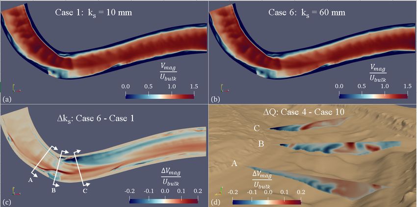
Figure 14. Comparison is shown for how different flow rates affect the velocity in the river.
Velocity magnitudes normalized by the mean flow velocity (Ubulk) at the water surface are shown
for flow rates of 92.5percent and 107.5 percent of the mean-flow rate (130.5 m3/s) in (a) and (b),
respectively. In (c), contours of the difference in surface velocity magnitudes for the two flow rates
are shown. The three cross-sections drawn with white lines are presented enlarged in (d). Flow is
from left to right.

Figure 15. Comparison is shown for how different equivalent roughness heights affect the velocity
in the river. Velocity magnitudes normalized by the mean flow velocity (Ubulk) at the water surface
are shown for two values of (10 mm and 60 mm) in (a) and (b), respectively. In (c), contours
of the difference in surface velocity magnitudes with two different values of 10 mm and 60 mm
are shown. The three cross-sections drawn with white lines are enlarged in (d). Flow is from left
to right.
 24

Figure 16. Contours of the LES-computed time-averaged velocity magnitudes normalized by the
mean-flow velocity (Ubulk) at the water surface (Vsurface) (a) and depth-averaged (Vavg) (b). (c) shows
contours of Vavg / Vsurface. (d) plots the variation of Vavg / Vsurface in the spanwise direction of the
river along the cross-sections A to D, as shown in (c).
 Thus far, we have demonstrated the strong yet somewhat unpredictable effect that both the
inflow discharge and equivalent roughness height can have on the velocity field of the river flow
in the study reach. Of principal interest in this study is the potential combined effect of these two
uncertain parameters on the LES results, as expressed by confidence intervals. In other words, we
seek to determine, with 95 percent confidence, the velocity magnitude of the river in the study
reach, considering the uncertainty associated with the flow discharge and equivalent bed
roughness. The computed velocities along selected cross-sections and velocity profile points were
sampled using the 11 LES cases to determine the joint effect. Specifically, Locations 2 to 5 were
selected along the mean cross-section location corresponding to the ADCP measurements, as
shown in Fig. 5, where 16 equally spaced depth-averaged velocities were determined and used for
the Uncertainty Quantification analysis. Similarly, the four-point locations (two along the cross-
section at Location 2 and two along the cross-section at Location 5 (Fig. 7) were selected for
samples of velocity profiles. Depending on flow depth, between 21 and 28 velocity magnitude
values were extracted from the LES results at each point location and labeled as VP1 to VP4.
These values were then used in the software program, Dakota, to determine the PCE coefficients
and Sobol indices. Subsequently, the PCE results were utilized to determine the confidence
intervals by randomly sampling 10,000 combinations of discharge and equivalent roughness
heights combinations using MC simulations. The range of variables used in the MC simulations
was as follows. Inflow discharge ranged uniformly within 10 percent of the mean discharge, and
 ! was varied uniformly between 10 mm and 65 mm. The results of these evaluations are presented
in Figs. 17 to 24.
 Considering the uncertainty in the depth-averaged velocity results for Location 2, which
mainly resides farthest upstream in the study reach, Fig. 17(b) shows that the computed results
from the LES correspond well with the recorded ADCP measurements. As seen, most of the ADCP
 25

measured data points fall within the 95 percent confidence limits. Considering that these
measurements reflect the average of only a few instantaneous measurements, readings outside of
the 95 percent confidence bands may be due to the error in the measurements. Conversely, since
Location 2 is near the inlet of the flow domain, it is likely that the velocity field imposed at the
inlet cross-plane (i.e., as the inlet boundary condition for the LES) does not accurately reflect the
proper boundary conditions. This is mainly due to the complexities associated with the meandering
bends upstream of the study reach, which were not considered.
 Furthermore, the computed velocities falling outside the 95 percent confidence bands are
located near the side banks, and these “outliers” tend to propagate downstream at the other
locations. The magnitude of the computational errors, however, tends to diminish in the
downstream direction. This trend would be expected because the LES results are gradually
corrected for the initial error in velocity distribution at the inlet as flow is conveyed downstream.
Quantifying the uncertainty caused by the distribution at the inlet is not possible without additional
bathymetry data, and a more extended study reach. Regarding the relative contribution to the
uncertainty, the Sobol indices in Fig. 17(c) show that the flow discharge almost entirely influences
the level of uncertainty in the depth-averaged velocities. This is evident in the Sobol indices that
uniformly exceed 0.9 throughout the study reach and, in all cross-sections, including depths
ranging from 2 m to over 7 m. This uniform impact of the flow rate on the overall uncertainty
could be better understood by employing a constant equivalent roughness height for all precursor
simulations, which were conducted to obtain the inlet boundary condition for the LESs. Since
Location 2 is nearest to the precursor flow, the full effect of varying the roughness height may
have not fully impacted the hydrodynamics of the river until farther downstream.

 26

Figure 17. The depth-averaged velocity magnitudes normalized by Ubulk in the spanwise direction
of the river at Location 2. (a) shows the study reach and the cross-section at Location 2. In (b), the
red solid-line shows the time-averaged LES results, circles are the instantaneously measured
ADCP data and dashed lines mark the 95 percent confidence intervals. In (c), The Sobol indices
for (red line), ! (blue line), and the combined effect of and ! (black line) are presented. The
Sobol indices mark the relative influence of each parameter on the overall uncertainty of the LES
results. For reference, the riverbed elevation (gray line) is plotted in (c).

 27

Location 3 is immediately downstream from the river bend and the confluence with
Sycamore Slough (Fig. 18(a)). Despite the strong secondary flow caused by the bend and the
additional (although minor) flow entering at the confluence, the computed LES results are still in
close agreement with the ADCP measured velocity field (Fig. 18(b)). As with Location 2, near
each bank, the measured depth-averaged velocities are slightly outside of the 95 percent
confidence bands. From the Sobol indices in Fig. 18(c), the uncertainty in the depth-averaged
results is almost entirely due to the uncertainty in the discharge near the center of the channel;
however, near the banks, a stronger influence of the bed roughness can be seen – particularly along
the left bank where the uncertainty due to the equivalent roughness height is more pronounced.
 At Locations 4, the cross-section is relatively uniform in shape (Fig. 19(c)) since it is
located at a cross-over point of the river thalweg. Location 5, on the other hand, is located farther
downstream of the study reach where the thalweg has shifted toward the left bank of the river (Fig.
20(c)). At both locations, the depth-averaged velocity measurements generally fall within the
uncertainty of the LES results except near the side banks. However, at Location 5, which is farthest
from the inlet precursor distribution, the measurements and numerical results are in closest
agreement. As for the previous locations, the Sobol indices show that near the center of the river,
the uncertainty in the computed results is strongly influenced by the uncertainty in the flow rate
with values typically exceeding 90 percent. However, near the side banks, the uncertainty is mainly
caused by the equivalent roughness height and ranges from 30 to 50 percent. It is worth noting that
the confidence intervals near the side banks show less uncertainty than in the center of the river.
Therefore, the increased Sobol index values do not necessarily indicate an absolute increase in the
uncertainty caused by the bed roughness but may only be a more significant percentage of the total
uncertainty in these regions.

 28

Figure 18. The depth-averaged velocity magnitudes normalized by Ubulk in the spanwise direction
of the river at Location 3. (a) shows the study reach and the cross-section at Location 3. In (b), the
red solid-line shows the time-averaged LES results, circles are the instantaneously measured
ADCP data and dashed lines mark the 95 percent confidence intervals. In (c), The Sobol indices
for (red line), ! (blue line), and the combined effect of and ! (black line) are presented. The
Sobol indices mark the relative influence of each parameter on the overall uncertainty of the LES
results. For reference, the riverbed elevation (gray line) is plotted in (c).

 29

Figure 19. The depth-averaged velocity magnitudes normalized by Ubulk in the spanwise direction
of the river at Location 4. (a) shows the study reach and the cross-section at Location 4. In (b), the
red solid-line shows the time-averaged LES results, circles are the instantaneously measured
ADCP data and dashed lines mark the 95 percent confidence intervals. In (c), The Sobol indices
for (red line), ! (blue line), and the combined effect of and ! (black line) are presented. The
Sobol indices mark the relative influence of each parameter on the overall uncertainty of the LES
results. For reference, the riverbed elevation (gray line) is plotted in (c).

 30

Figure 20. The depth-averaged velocity magnitudes normalized by Ubulk in the spanwise direction
of the river at Location 5. (a) shows the study reach and the cross-section at Location 5. In (b), the
red solid-line shows the time-averaged LES results, circles are the instantaneously measured
ADCP data and dashed lines mark the 95 percent confidence intervals. In (c), The Sobol indices
for (red line), ! (blue line), and the combined effect of and ! (black line) are presented. The
Sobol indices mark the relative influence of each parameter on the overall uncertainty of the LES
results. For reference, the riverbed elevation (gray line) is plotted in (c).

 31

The velocity profiles in the water column were also analyzed using the same UQ
methodology to define the confidence bands and Sobol indices of the LES results at 4 locations
within the study reach. Locations VP1 and VP2 are along the outer bank at the entrance to the
meander bend on the same cross-section at Location 2 discussed above. For these two computed
velocity profiles, most of the measured velocity data does not fall within the 95 percent confidence
intervals. We conjecture that this may be primarily due to the measured values, which reflect only
instantaneous velocity readings. While the depth-averaged ADCP readings in the spanwise
directions were also computed by averaging only a few instantaneous readings, the depth-
averaging process itself helps smooth out the instantaneous fluctuations by averaging the ensemble
of values over the entire water column. However, the velocity profiles in the vertical direction do
not have this same advantage and show only the average of 3 or 4 instantaneous readings. To better
assess this error, one would need to make stationary measurements over several minutes to account
for the various turbulent structures passing through a given point. We note that such stationary
measurements in the field are extremely difficult. Locations VP3 and VP4 fall along the cross-
section at Location 5, with VP3 and VP4 being located near the left and right banks, respectively
(Fig. 23 (a) and (b)). At these two locations, the ADCP measurement data agree more closely with
the LES results. This improved agreement may be due to the fact that these points are far away
from the inlet and strong secondary effects due to the bend. For each case, the Sobol indices for
 ! increases appreciable from less than 5 percent near mid-depth to between 15 to 40 percent near
the bed. This increase influence of equivalent roughness height on the uncertainty near the bed
seems reasonable since the value for ! is directly applied to the wall model to reconstruct the
velocity field of the computational nodes near the bed. However, it is also noted that the confidence
limits near the riverbed are very small for each of the four vertical profiles indicating the
uncertainty associated with and ! are primarily experienced away from the bed. In this light,
the influence of ! on the uncertainty should be recognized as higher relative to and not as
causing greater uncertainty in an absolute sense.

 32

Figure 21. The vertical profile of velocity magnitude normalized by Ubulk at point VP1. (a) and (b)
illustrate the location of the VP1 over the riverbed. In (b), the red line shows the time-averaged
LES results, dashed black lines mark the 95 percent confidence bands, and circles represent the
instantaneous ADCP data. (d) depicts the Sobol indices for , ! , and combined effect of and
 ! , showing each parameter's relative influence on the overall uncertainty.

 33

Figure 22. The vertical profile of velocity magnitude normalized by Ubulk at point VP2. (a) and (b)
illustrate the location of the VP1 over the riverbed. In (b), the red line shows the time-averaged
LES results, dashed black lines mark the 95 percent confidence bands, and circles represent the
instantaneous ADCP data. (d) depicts the Sobol indices for , ! , and combined effect of and
 ! , showing each parameter's relative influence on the overall uncertainty.

 34