A triple tree-ring constraint for tree growth and physiology in a global land surface model
←
→
Page content transcription
If your browser does not render page correctly, please read the page content below
Biogeosciences, 18, 3781–3803, 2021
https://doi.org/10.5194/bg-18-3781-2021
© Author(s) 2021. This work is distributed under
the Creative Commons Attribution 4.0 License.

A triple tree-ring constraint for tree growth and physiology
in a global land surface model
Jonathan Barichivich1,2 , Philippe Peylin1 , Thomas Launois1 , Valerie Daux1 , Camille Risi3 , Jina Jeong4 , and
Sebastiaan Luyssaert4
1 Laboratoire des Sciences du Climat et de l’Environnement (LSCE), Gif sur Yvette, France
2 Instituto
          de Geografía, Pontificia Universidad Católica de Valparaíso, Valparaíso, Chile
3 Laboratoire de Météorologie Dynamique (LMD), Paris, France
4 Department of Ecological Sciences, VU University, 1081HV Amsterdam, the Netherlands

Correspondence: Jonathan Barichivich (jonathan.barichivich@ipsl.lsce.fr)

Received: 28 November 2020 – Discussion started: 10 December 2020
Revised: 18 May 2021 – Accepted: 22 May 2021 – Published: 24 June 2021

Abstract. Annually resolved tree-ring records extending            models as demonstrated here should guide model improve-
back to pre-industrial conditions have the potential to con-       ments and contribute towards reducing current uncertainties
strain the responses of global land surface models at interan-     in forest carbon and water cycling.
nual to centennial timescales. Here, we demonstrate a frame-
work to simultaneously constrain the representation of tree
growth and physiology in the ORCHIDEE global land sur-
face model using the simulated variability of tree-ring width
and carbon (113 C) and oxygen (δ 18 O) stable isotopes in six      1   Introduction
sites in boreal and temperate Europe. We exploit the result-
ing tree-ring triplet to derive integrative constraints for leaf   A major challenge for the land surface model (LSM) com-
physiology and growth from well-known mechanistic rela-            ponent of Earth system models is to accurately simulate the
tionships among the variables. ORCHIDEE simulates 113 C            historical and future dynamical coupling between the global
(r = 0.31–0.80) and δ 18 O (r = 0.36–0.74) better than tree-       biosphere and climate (Friedlingstein et al., 2014). Although
ring width (r < 0.55), with an overall skill similar to that       LSMs are skillful at reproducing short-term (< 20 years)
of a tree-ring model (MAIDENiso) and another isotope-              contemporary observations of plant water and carbon cy-
enabled global vegetation model (LPX-Bern). The compar-            cling, their simulated responses to environmental changes at
ison with tree-ring data showed that growth variability is not     longer timescales from decades to centuries are still highly
well represented in ORCHIDEE and that the parameteriza-            uncertain and contribute to the spread in current climate
tion of leaf-level physiological responses (stomatal control)      change projections (Ciais et al., 2013; Friedlingstein et al.,
to drought stress in the temperate region can be constrained       2014). Some of these models project that the terrestrial bio-
using the interannual variability of tree-ring stable isotopes.    sphere will continue behaving as a carbon sink of anthro-
The representation of carbon storage and remobilization dy-        pogenic emissions during the course of the century, while
namics emerged as a critical process to improve the realism        others simulate that it will turn into an additional carbon
of simulated growth variability, temporal carryover, and re-       source to the atmosphere that will accelerate climate change
covery of forest ecosystems after climate extremes. Simu-          (Friedlingstein et al., 2006; Jones et al., 2013; Friedlingstein
lated forest gross primary productivity (GPP) correlates with      et al., 2014). The uncertainties in simulated long-term trends
simulated tree-ring 113 C and δ 18 O variability, but the origin   are also evident for the water cycle and over the historical
of the correlations with tree-ring δ 18 O is not entirely phys-    period (Frank et al., 2015; Phillips et al., 2019). The lack of
iological. The integration of tree-ring data and land surface      a general agreement on the historical and future long-term
                                                                   responses of the terrestrial biosphere in land surface mod-

Published by Copernicus Publications on behalf of the European Geosciences Union.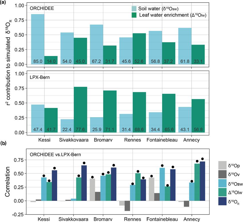
3782                                                                          J. Barichivich et al.: Tree rings in ORCHIDEE

els thus limits confidence in future climate projections (Ciais    ple carbon-source approach and consider it to be the differ-
et al., 2013).                                                     ence between instantaneous photosynthetic carbon assimila-
    The development, parameterization, and evaluation of cur-      tion and respiration. Sink processes of wood formation, em-
rent land surface models have been based on a handful of ma-       phasized in tree-level models (Vaganov et al., 2011), are ne-
nipulative experiments (Ainsworth and Long, 2005; Smith            glected (Fatichi et al., 2014). Reserve pools of labile carbon
et al., 2015; Andresen et al., 2016; Song et al., 2019), a         have only recently been considered because of the need to re-
quasi-global network of eddy-covariance observations (Bal-         alistically represent continued forest growth when photosyn-
docchi, 2019), Earth observations (Orth et al., 2017), and for-    thesis is suppressed by environmental stresses (Naudts et al.,
est inventories (Bellassen et al., 2011) covering the last few     2015; Vuichard et al., 2019; Jones et al., 2020). Currently
decades. Most of these data streams are not able to reveal         there is no global land surface model with the capability
the temporal evolution of plant responses to global change         to explicitly simulate tree-ring width. Nevertheless, tree-ring
factors at multi-decadal and longer timescales, where mech-        width data have been used as an indirect benchmark for the
anistic understanding on how trees perish or adapt to en-          interannual variability of simulated net primary productivity
vironmental change is still limited (McDowell et al., 2008;        in some global land surface models (Rammig et al., 2015;
Cailleret et al., 2018). Tree-ring width and their carbon          Churakova et al., 2016). In contrast to ring width, tree-ring
(δ 13 C) and oxygen (δ 18 O) stable isotope data are increas-      δ 13 C or δ 18 O stable isotopes have already been incorporated
ingly being used to address the lack of direct observations        in some global land surface models such as FOREST-BGC
on long-term changes in plant physiology and growth with           (Panek and Waring, 1997), ORCHIDEE (Shi et al., 2011;
global change (Huang et al., 2007; Frank et al., 2015; Gi-         Churakova et al., 2016; Risi et al., 2016), JULES (Bodin
rardin et al., 2016; Babst et al., 2018; de Boer et al., 2019;     et al., 2013), LPX-Bern (Saurer et al., 2014; Keel et al., 2016;
Lavergne et al., 2020) and could provide the much needed           Keller et al., 2017), and CLM4.5 (Raczka et al., 2016; Keller
long-term benchmark for land surface models (Zuidema               et al., 2017).
et al., 2018).                                                        An enormous benefit of explicitly modeling tree-ring
    In recent decades, some dendrochronological and forest         width and stable isotopes in the global land surface mod-
process-based models have successfully integrated the simu-        els is the ability to directly compare readily available tree-
lation of tree-ring width with stable isotopes in order to in-     ring data to modeled data. Thus, the global models can be
terpret measurements and improve simulated tree water sta-         evaluated and improved with freely available worldwide tree-
tus, photosynthesis, and growth (Fritts et al., 1999; Hem-         ring data found, for example, in the International Tree-ring
ming et al., 2001; Ogée et al., 2009; Eglin et al., 2010; Da-      Data Bank (ITRDB) and tree-ring laboratories around the
nis et al., 2012; Wei et al., 2014; Ulrich et al., 2019). Radial   world. Furthermore, the interpretation of these tree-ring data
growth is represented with decreasing complexity from tree         can be supported by model simulations. The comparison of
to stand-level models, considering different degrees of inte-      simulated δ 13 C and derived physiological indicators such as
gration of controls from sources (photosynthesis and alloca-       the carbon isotopic discrimination (113 C) by plants and the
tion) and sinks (cell growth) of carbon in the trees (Vaganov      intrinsic water use efficiency (iWUE) with direct tree-ring
et al., 2011; Körner, 2015). The tree-ring community has           isotopic measurements has helped benchmark stomatal re-
developed a detailed source–sink representation of radial          sponses to drought stress and rising atmospheric CO2 con-
growth for conifers as the product of daily cambial dynam-         centrations in the global models (Panek and Waring, 1997;
ics and wood formation (i.e., cell division, enlargement, and      Bodin et al., 2013; Saurer et al., 2014; Keller et al., 2017).
wall thickening), coupled or not to a full representation of       Simulated δ 18 O has been used to evaluate the representation
tree-level photosynthesis and carbon allocation (Fritts et al.,    of hydrological processes along the soil–plant–atmosphere
1999; Hemming et al., 2001; Vaganov et al., 2011; Drew and         continuum (Risi et al., 2016) and interpret the variability in
Downes, 2015). Stand-level forest models parameterize ra-          tree-ring δ 18 O data in terms of climatic drivers and source
dial growth of conifers and angiosperms as a direct depen-         water δ 18 O (Shi et al., 2011; Keel et al., 2016; Churakova
dency of photosynthesis, using the allocation of photosyn-         et al., 2016). The interannual variability of tree-ring δ 13 C
thates and tree allometry (Deleuze et al., 2004; Misson, 2004;     and δ 18 O has been shown to correlate with local eddy-
Sato et al., 2007; Li et al., 2014). A well-known stand-level      covariance measurements of forest productivity (Belmecheri
tree-ring model using this approach is MAIDENiso (Danis            et al., 2014; Tei et al., 2019). A recent study showed that
et al., 2012; Lavergne et al., 2017), which has the unique         the relationship holds at a regional scale and is stronger for
triple capability to simulate radial growth and oxygen and         δ 18 O than δ 13 C and tree-ring width (Levesque et al., 2019),
carbon isotopic ratios in tree rings.                              suggesting that tree-ring isotopic variability might integrate
    The representation of tree biomass growth in global land       large-scale physiological signals useful to evaluate global
surface models is still rudimentary and is one of the criti-       carbon cycle models. Yet, stable isotope–productivity rela-
cal areas where much improvement is needed (Fatichi et al.,        tionships have not been studied in this type of model.
2014; Körner, 2015; Jones et al., 2020). Like stand-level             Empirical tree-ring studies frequently combine δ 18 O and
models, most global models represent growth using a sim-             13
                                                                   δ C as a means to mechanistically interpret plant physi-

Biogeosciences, 18, 3781–3803, 2021                                                   https://doi.org/10.5194/bg-18-3781-2021
J. Barichivich et al.: Tree rings in ORCHIDEE                                                                                  3783

ological responses (Saurer et al., 1997; Scheidegger et al.,         gether with respiration, the energy balance and hydrological
2000; Barnard et al., 2012; Roden and Farquhar, 2012; Sze-           processes are simulated at a half-hourly time step, which is
jner et al., 2020). In contrast, most of the studies with land       the typical resolution of eddy-covariance measurements of
surface models have focused on the simulation and evalu-             carbon and water fluxes (Baldocchi et al., 2001). Leaf gas
ation of a single tree-ring variable (Saurer et al., 2014; Keel      exchange is simulated by coupling the photosynthesis model
et al., 2016; Keller et al., 2017). Key developments in the OR-      with the stomatal conductance model of Ball et al. (1987).
CHIDEE global land surface model now allow the explicit              The CO2 demand is determined as the minimum of Rubisco
simulation of radial growth (Bellassen et al., 2010; Naudts          carboxylation and RuBP regeneration, while CO2 supply de-
et al., 2015; Jeong et al., 2020) and carbon and oxygen com-         pends on the difference in CO2 concentration between the
position in tree-ring cellulose (Risi et al., 2016) as done in the   air outside the leaf and the carboxylation sites. Carbon allo-
MAIDENiso tree-ring model (Danis et al., 2012). This offers          cation to the different vegetation pools, phenology, and mor-
the opportunity to explore how multiple tree-ring variables          tality are calculated at a daily time step.
can be used to constrain the long-term plant responses sim-             Soil hydrology is modeled using a surface and a deep
ulated by global land surface models and identify processes          reservoir (Choisnel et al., 1995). Water enters the surface
that need to be better represented or parameterized.                 layer via throughfall, snowmelt, and dew and frost. Water can
   The aims of this study are to (i) integrate key develop-          leave the soil reservoir through transpiration, bare soil evapo-
ments and identify the critical processes to concurrently sim-       ration, surface runoff, and drainage. Plant water stress is cal-
ulate the interannual variability of tree-ring width and its car-    culated at half-hourly time steps as a function of soil water
bon (113 C) and oxygen stable isotopes in the ORCHIDEE               content (McMurtrie et al., 1990) weighted by root mass. Wa-
global land surface model, (ii) develop a conceptual triple          ter stress reduces transpiration through a direct reduction of
tree-ring constraint for simulated growth and physiology that        stomatal conductance as soil moisture depletes.
exploits the mechanistic relationships among tree-ring vari-            The key developments used for simulating tree-ring pa-
ables, and (iii) evaluate the simulated relationships between        rameters include the addition of a forest management mod-
productivity and tree-ring carbon and oxygen stable isotopes.        ule (Bellassen et al., 2010) and the simulation of oxygen
We first assess and compare the ability of ORCHIDEE and              stable isotope ratios along the soil–plant–atmosphere contin-
MAIDENiso models to simulate 20th century tree-ring width            uum (Risi et al., 2016). The model code used in this study
and isotopic variability and their inter-relationships in the        (SVN r898 version) precedes the current code that merged
Fontainebleau forest in France. Then, we run ORCHIDEE in             the nitrogen cycle and canopy structure in ORCHIDEE r5698
five other sites along a climate gradient from boreal Finland        (Naudts et al., 2015; Vuichard et al., 2019), where the tree-
to temperate France, and we compare its ability to simulate          ring functionality will also be reported (Jeong et al., 2020).
δ 18 O variability in the gradient with that of the LPX-Bern
global vegetation model (Keel et al., 2016). The simulated           2.1.1   Tree-ring width
relationships between isotopic variability and productivity in
ORCHIDEE are also evaluated along the gradient.                      The forest management module explicitly simulates the tem-
                                                                     poral trajectory of stem growth of trees in a size-structured
                                                                     forest stand. The size structure of the stand is prescribed by
2     Model and evaluation data                                      defining a starting density of trees per hectare distributed
                                                                     across a number of stem diameter size classes, typically
2.1    Model description                                             following an inverted-J distribution. Initial tree height and
                                                                     biomass are obtained by allometric relationships with stem
The global land surface model ORCHIDEE (Krinner et al.,              diameter (Bellassen et al., 2010). For each PFT, photosyn-
2005) is the terrestrial component of the IPSL (Institut Pierre      thesis and net primary production (NPP) are computed at the
Simon Laplace) Earth system model (Dufresne et al., 2013;            stand level at half-hourly and daily steps, respectively.
Boucher et al., 2020). ORCHIDEE simulates the half-hourly               At the end of the year, accumulated woody NPP increment
exchange of energy, carbon, and water between the terrestrial        is allocated across the different diameter classes following an
biosphere and the atmosphere, either coupled with the LMDz           empirical competition rule for evenly aged stands (Deleuze
(Laboratoire de Météorologie Dynamique Zoom) general cir-            et al., 2004). A greater NPP share is allocated to larger domi-
culation model (Hourdin et al., 2006) or forced by observed          nant trees compared to smaller less vigorous trees, emulating
meteorology.                                                         the competition for light and resources within the stand. The
   The global forests are represented by eight plant functional      absolute annual stem growth increment in the allocation rule
types (PFTs) described by a common set of governing equa-            is determined by a parameter (λ) that defines the slope be-
tions with specific parameter values, with the only exception        tween the fraction of NPP allocated to each diameter class
being some PFT-specific phenology representations (Krinner           and the mean diameter of the class. A second parameter (σ )
et al., 2005). Canopy photosynthesis is based on the leaf-level      represents a diameter threshold below which less vigorous
photosynthesis formulation of Farquhar et al. (1980), and to-        trees receive only a fixed part of the yearly stand NPP incre-

https://doi.org/10.5194/bg-18-3781-2021                                                     Biogeosciences, 18, 3781–3803, 2021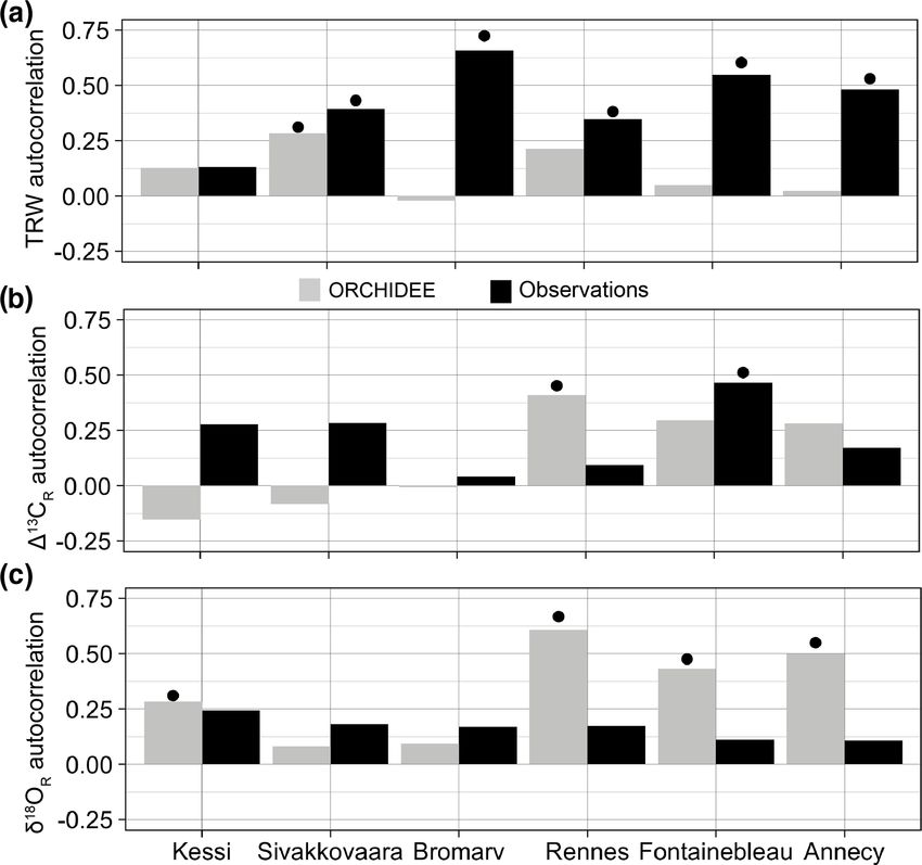
3784                                                                            J. Barichivich et al.: Tree rings in ORCHIDEE

ment. The stem growth of the largest and smallest trees is           from measured δ 13 C in tree-ring cellulose (Francey and
tracked individually through the entire simulation (Bellassen        Farquhar, 1982). For simplicity, it assumes that further
et al., 2010).                                                       post-photosynthetic fractionation during photo- and dark-
   Simulated tree-ring width (i.e., radial growth) for each di-      respiration and carbohydrate remobilization and storage is
ameter class was computed from annual increments in stem             negligible. Although these processes normally have an im-
circumference as follows:                                            portant impact on whole-ring cellulose isotopic composition
          Circt − Circt−1                                            (Gessler et al., 2009; Werner et al., 2012), at least the im-
TRWt =                    ,                                   (1)    pact of carbon remobilization is minimal in the latewood
                2π
                                                                     component of tree rings (Helle and Schleser, 2004). The ci
where TRWt is the annual tree-ring width in millimeters for          term in Eq. (2) integrates the gas exchange dynamics (i.e.,
the year t, and Circt and Circt−1 are the stem circumfer-            stomatal conductance and photosynthesis) simulated by the
ences for the current year and the previous year, respectively.      model as a complex function of micrometeorological vari-
The annual ring widths simulated in this scheme account for          ability, seasonal water stress, and the long-term warming and
the size-related trend in stem growth increment and PFT-             increase in ca . Hence, despite its simplicity, simulated carbon
specific tree allometry, providing a mean representation of          discrimination using Eq. (2) has been shown to be valuable to
radial growth for trees across a range of sizes that can be          constrain the integrated environmental response of land sur-
meaningfully compared with measured tree-ring width data.            face models using carbon discrimination derived from tree-
However, in this formulation tree-ring width variability de-         ring δ 13 C measurements (e.g., Bodin et al., 2013; Churakova
pends only on direct GPP allocation (i.e., it is a carbon-           et al., 2016; Keel et al., 2016).
source-driven process) and does not consider the dynamics
of carbon storage or wood formation processes that can ac-           2.1.3   Tree-ring oxygen isotopes
count for a large fraction of observed interannual tree-ring
width variation (Misson, 2004).                                      The δ 18 O signature in tree-ring cellulose primarily reflects
                                                                     the isotopic composition of soil water and the evaporative en-
2.1.2   Tree-ring carbon isotopes                                    richment of leaf water due to transpiration, but other mixing
                                                                     and biochemical fractionation processes during water trans-
To eliminate the effect of δ 13 C of atmospheric CO2 and pre-
                                                                     port along the soil–plant–atmosphere continuum also con-
serve only the effects of plant metabolic processes, the 13 C
                                                                     tribute to the final δ 18 O signature (Gessler et al., 2014). The
enrichment of plant organic material is usually expressed in
                                                                     δ 18 O isotopic composition of the source water used by plants
terms of the carbon isotope discrimination (113 C). Differ-
                                                                     may originate from rainfall or groundwater, while the δ 18 O
ences between the 13 C enrichment of atmospheric CO2 and
                                                                     isotopic enrichment of leaf water depends strongly on va-
plant material are attributed to discriminatory processes dur-
                                                                     por pressure deficit (i.e., the ratio of the vapor pressure in
ing photosynthesis.
                                                                     the atmosphere and the intercellular spaces of the leaves) or
   Photosynthetic carbon isotope discrimination was esti-
                                                                     relative humidity (Farquhar et al., 1998; Scheidegger et al.,
mated at half-hourly time steps using the simple formulation
                                                                     2000).
of Farquhar et al. (1982) for C3 plants:
                                                                        The δ 18 O fractionation and mixing processes in all water
                      ci                                             pools and fluxes along the soil–plant–atmosphere continuum
113 C = a + (b − a)      ,                                    (2)
                      ca                                             (Risi et al., 2016) are represented following a similar formu-
where a (4.4 ‰) is the kinetic discrimination associated with        lation as in other isotope-enabled global land surface models
diffusion between free air and the stomatal cavity, b (27 ‰) is      (Aleinov and Schmidt, 2006; Haese et al., 2013). The iso-
the fractionation during CO2 fixation by the Rubisco enzyme          topic composition of precipitation and near-surface water va-
(Farquhar et al., 1982; Cernusak et al., 2013), ci is the leaf in-   por have to be prescribed monthly when running the model
ternal CO2 concentration simulated by ORCHIDEE, and ca               stand-alone or are simulated by the LMDz general circulation
is the atmospheric CO2 concentration prescribed from mea-            model in coupled simulations. Precipitation reaching the soil
surements. Annual tree-ring carbon discrimination (113 CR )          surface or intercepting the canopy fractionates during evap-
was then calculated as the mean of the half-hourly discrimi-         oration according to the Craig and Gordon equation (Craig
nation values in the above-ground biomass weighted by gross          and Gordon, 1965), which generically describes the prefer-
primary productivity (GPP) between the start (SOS) and the           ential evaporation of the lighter isotope of a free water body
end (EOS) of the growing season:                                     at steady state.
                                                                        The resulting isotopic composition of soil water and mix-
                              EOS                                    ing are parameterized as a vertical profile to overcome the
                  1           X
113 CR = PEOS                        113 C(n) × GPP(n) .      (3)    limitation of depth resolution in the two-layer representation
             n=SOS GPP(n) n=SOS
                                                                     of soil in the model. No isotopic fractionation is assumed to
  This formulation for carbon discrimination is commonly             occur during absorption of soil water by roots, and thus the
used as a simple approximation for discrimination derived            isotopic signature of xylem water is the same as that of soil

Biogeosciences, 18, 3781–3803, 2021                                                     https://doi.org/10.5194/bg-18-3781-2021
J. Barichivich et al.: Tree rings in ORCHIDEE 3785
water. The isotopic composition of leaf water at the evapo- A model evaluation across a network of 10 sites in Europe
ration sites (δ 18 Oe ) is diagnosed by inverting the Craig and and North America shows that this representation is able to
Gordon (1965) equation: reproduce the main features of the seasonal and vertical vari-
ations in soil water isotope content, as well as the seasonal
δ 18 Oe = α αk × (1 − h) × δ 18 Osw + h × δ 18 Ov , (4) isotopic signals in stem and leaf water (Risi et al., 2016). The
isotopic variability simulated by ORCHIDEE has been used
where δ 18 Osw is the isotopic composition of soil water taken to interpret local climatic signals in tree-ring δ 18 O records
up by the roots integrating older soil water and recent precip- (Shi et al., 2011; Churakova et al., 2016) and to investigate
itation, δ 18 Ov is the isotopic composition of atmospheric wa- regional and global isotopic signatures of continental recy-
ter vapor, α is the equilibrium fractionation due to the phase cling (Risi et al., 2013).
change from liquid water to vapor, αk is the kinetic fraction-
ation due to diffusion of vapor into unsaturated air, and h is 2.2 Tree-ring data
the relative humidity normalized to surface temperature.
Isotopic enrichment of leaf water in the mesophyll Six previously published tree-ring datasets in northern and
(δ 18 Olw ) results from mixing between isotopically enriched western Europe with simultaneous measurements of ring
leaf water at the evaporative site and depleted xylem water width and δ 13 C and δ 18 O compositions were used to eval-
(δ 18 Oxw ) through the so-called Péclet effect: uate the skill of the model along a climate gradient (Table 1).
The three northernmost sites are located in the temperature-
δ 18 Olw = δ 18 Oe × f + δ 18 Oxw × (1 − f ), (5) limited boreal region in Finland and have chronologies of
where f = (1 − e−P )/P is a coefficient that decreases as the ring width and δ 13 C and δ 18 O composition for Scotch pine
Péclet effect increases, with P = (E × L)/(W × D) as the (Kessi and Sivakkovaara; Hilasvuori et al., 2009) and pe-
Péclet parameter. E is the transpiration rate per leaf area, L dunculate oak (Bromarv; Hilasvuori and Berninger, 2010).
is the effective diffusion length, and W is the leaf water con- The remaining three sites are located in France and rep-
tent per leaf volume. In order to keep the model as simple resent moisture-sensitive temperate forests of sessile oak
as possible, L was set to 8 mm and W was assumed to be (Fontainebleau; Etien et al., 2009) and pedunculate oak
103 kg m−3 for all PFTs following Risi et al. (2016). Admit- (Rennes and Annecy; Raffalli-Delerce et al., 2004; Danis
tedly, constant L is a major assumption and source of uncer- et al., 2006). In all sites, except Annecy, the available ring
tainty for global models (Keel et al., 2016; Risi et al., 2016) width and δ 13 C and δ 18 O chronologies cover the common
since it is highly variable between species and also depends period 1960–2000.
on climate conditions and leaf anatomy, morphology, and age The tree-ring width measurement series available for each
(Barnard et al., 2007; Roden et al., 2015). The value used site were standardized by dividing each series by its mean
for L was obtained from an optimization of simulated diur- ring width (Cook et al., 1990). The resulting series of tree-
nal isotopic cycles against observations at mid-latitude sites ring width indices were averaged together to produce a mean
(Risi et al., 2016). site chronology composed by 7 to 28 trees (Table 1). This
Half-hourly tree-ring cellulose isotopic composition simple standardization method allows the computation of av-
(δ 18 Ocell ) is calculated from the isotopic composition of leaf erage tree-ring chronologies without the average being dom-
water (δ 18 Olw ) and xylem water (δ 18 Oxw ) following the for- inated by the faster growing trees with wider rings. Depend-
mulation of Anderson et al. (2002): ing on the site, four to nine trees were selected to develop car-
bon (δ 13 CR ) and oxygen (δ 18 OR ) stable isotope chronologies
δ 18 Ocell = f 0 × δ 18 Oxw + (1 − f 0) × δ 18 Olw × (1 + ), (6) by pooling rings from the selected trees (Table 1) and using
standard methods for cellulose extraction and measurement
where f 0 is the fraction of exchange with xylem water prior of the isotopic ratios (McCarroll and Loader, 2004; Daux
to cellulose synthesis, which reduces the imprint of leaf wa- et al., 2018). For oaks, earlywood and latewood sections were
ter on cellulose. For δ 18 O this exchange is estimated to be separated, but only latewood was processed. For pine, the
0.42 based on the best-fit relationship under controlled ex- carbon and oxygen isotopic compositions were measured for
periments (Roden et al., 2000). The parameter is the bio- the whole ring.
chemical fractionation factor during cellulose formation as- Tree-ring carbon discrimination was computed by sub-
sociated with water carbonyl interactions and is estimated to tracting the stable carbon isotope composition of the atmo-
be 27 ‰ (DeNiro and Epstein, 1979; Stenberg and DeNiro, sphere (δ 13 Ca ) from the measurements using the expression
1983). of Farquhar et al. (1982):
An estimate of growing season tree-ring isotopic compo-
sition (δ 18 OR ) is obtained by weighting δ 18 Ocell by GPP as δ 13 Ca − δ 13 CR
113 CR = . (8)
done for 113 CR in Eq. (3): 13
CR
1 + δ1000
EOS
1 Data for δ 13 Ca were obtained from McCarroll and Loader
X
δ 18 OR = PEOS δ 18 Ocell (n) × GPP(n) . (7)
n=SOS GPP(n) n=SOS
(2004) for the period 1901–2000.
https://doi.org/10.5194/bg-18-3781-2021 Biogeosciences, 18, 3781–3803, 20213786 J. Barichivich et al.: Tree rings in ORCHIDEE
Table 1. Location and characteristics of the six tree-ring sites used for model evaluation. The ORCHIDEE plant functional types (PFTs)
corresponding to the sites are boreal needleleaf evergreen (BoNE), boreal broadleaf summergreen (BoBS), and temperate broadleaf summer-
green (TeBS).
Site
Kessi Sivakkovaara Bromarv Rennes Fontainebleau Annecy
Country Finland Finland Finland France France France
Species Pine Pine Oak Oak Oak Oak
ORCHIDEE PFT BoNE BoNE BoBS TeBS TeBS TeBS
Latitude 68.6 62.5 60.0 48.1 48.4 45.9
Longitude 28.2 31.2 23.0 −1.7 2.7 6.2
Elevation (m) 159 200 5 70 100 450
Stand age (years) 400 400 150 120 120 70
Stand density (trees ha−1 ) – – – 240 140 40
No. of trees for tree-ring width 16 28 7 28 15 13
No. of trees for tree-ring isotopes 4 4 4 4 4 9
Soil type Sandy loam Sandy loam Sandy loam Loam Calcareous loam Clay loam
Soil depth (m) < 0.5 < 0.5 0.5 1.5 1.0 –
Annual precipitation (mm) 390 582 502 677 678 906
Annual mean minimum temperature (◦ C) −4.8 −1.8 4.5 7.6 6.4 6.6
Annual mean maximum temperature (◦ C) 4.3 5.8 9.1 16.0 15.4 16.2
2.3 Simulations is decoupled from instantaneous photosynthesis by a labile
carbon pool, which allows the model to reproduce the tem-
The model was run at each tree-ring site over the period poral autocorrelation in tree rings (Misson, 2004). The sim-
1901–2000 using as meteorological forcing the nearest 0.5◦ ulation was produced using a site-specific calibration and in-
grid of the 6-hourly CRU-NCEP dataset (Viovy, 2014). This cludes tree-ring width, δ 13 C, and δ 18 O over the period 1953–
gridded forcing dataset is a statistical merging of the monthly 2000 as described in Danis et al. (2012). The daily δ 18 Op
CRU TS station-based dataset of the Climate Research Unit and δ 18 Ov forcings were obtained by using a linear regres-
(New et al., 2000) with the atmospheric reanalysis from the sion based on daily mean air temperature and precipitation
National Centers for Environmental Prediction (NCEP). The from two nearby stations as predictors, with coefficients ob-
corresponding soil type and vegetation PFT were prescribed tained from the nearest isotopic observations in Saclay.
for the sites (Table 1). Monthly δ 18 O composition of precip- In addition, tree-ring δ 18 O simulated with the LPX-Bern
itation (δ 18 Op ) and water vapor (δ 18 Ov ) was obtained from Dynamic Global Vegetation Model (Keel et al., 2016) was
the nearest grid of a global simulation of the isotope-enabled extracted for each site from a published global simula-
LMDz general circulation model nudged by an atmospheric tion available for the period 1960–2012 at 3.75◦ × 2.75◦
reanalysis over the period 1890–2007 (Risi et al., 2010). (dataset available at https://www.climate.unibe.ch, last ac-
Biomass and soil carbon pools were initialized to steady- cess: 18 June 2021). This simulation was obtained by forcing
state equilibrium by a 5000-year spinup obtained by cycling LPX-Bern with monthly soil water δ 18 O (δ 18 Osw ), δ 18 Ov ,
over the meteorology for the period 1901–1910. The model and relative humidity data from a simulation with the coupled
was then run over the period 1901–2000 using observed CO2 atmosphere–land surface model ECHAM5-JSBACH driven
and an initial tree density of 1000 trees per hectare to ap- by observed sea surface temperature (Haese et al., 2013;
proach current forest age and density following tree mortality Keel et al., 2016). LPX-Bern uses the Péclet modified Craig–
over time due to self-thinning. Gordon model to calculate daily δ 18 O in leaf water together
In order to benchmark the triple tree-ring ability of OR- with the formulation of Roden–Lin–Ehleringer (Roden et al.,
CHIDEE, a simulation of the MAIDENiso tree-ring model 2000) to determine δ 18 O in tree-ring cellulose.
for the Fontainebleau forest was obtained from an earlier
study (Danis et al., 2012). The model simulates tree-ring 2.4 Model–data comparison
δ 13 C and δ 18 O stable isotopes using the formulation of Lloyd
and Farquhar (1994) and the Craig–Gordon model (Craig and The ability of ORCHIDEE to simulate the interannual vari-
Gordon, 1965), respectively. Ring width is parameterized as ability of the three tree-ring parameters over the course of
the annual stem growth increment based on daily carbon al- the 20th century was first evaluated in the Fontainebleau for-
location to leaves, stem, roots, and storage as a function of est (Table 1). Fontainebleau is a well-studied tree-ring site
climate, soil water balance, and atmospheric CO2 . Growth in France (Michelot et al., 2011, 2012; Daux et al., 2018)
Biogeosciences, 18, 3781–3803, 2021 https://doi.org/10.5194/bg-18-3781-2021J. Barichivich et al.: Tree rings in ORCHIDEE 3787 and it has been used to evaluate the MAIDENiso tree-ring 2020). This visualization device extends the dual isotope model (Danis et al., 2012). We compared our simulation of conceptual model of Scheidegger et al. (2000) to illustrate the ring width, 113 C, and δ 18 O for this site with the simulation mechanistic information content of the triple tree-ring con- of MAIDENiso over the period 1953–2000. Then, the evalu- straint for models introduced in this study. It neatly reveals ation was conducted for the rest of the sites over the common the complex association of tree growth with gas exchange period 1960–2000, except in Annecy where a shorter span of inferred from stable isotopes in both observations and mod- the observations limited the model–data comparison to the els. period 1971–2000. To disentangle the relative importance of source wa- A simulated tree-ring width chronology was derived for ter (δ 18 Osw ) and leaf water enrichment above source wa- each site by dividing the simulated tree-ring width series of ter (118 Olw = δ 18 Olw − δ 18 Osw ) between May and August the largest model tree by its mean. Since growth allocation in determining the variability of δ 18 OR simulated by OR- in the model increases almost linearly with stem size, the CHIDEE and LPX-Bern, we used the Lindeman–Merenda– absolute annual ring width varies among stem size classes, Gold (LMG) method (Grömping, 2006). This linear decom- but its interannual variability remains similar across all size position method quantifies the contribution of different cor- classes; thus the choice of size class does not affect the stan- related regressors (here δ 18 Osw and 118 Olw ) to the total r 2 dardized variability. The standardization removes the effect of a multiple linear regression model. of stem size class and conserves the interannual and longer variability but does not remove the juvenile effect in tree-ring width. However, the juvenile trend in simulated and observed 3 Results ring width does not affect the evaluation period (1960–2000) because at this time trees were already mature canopy indi- 3.1 A triple tree-ring constraint for ORCHIDEE and viduals with their radial growth fluctuating around the mean. MAIDENiso in Fontainebleau Simulated δ 18 O and 113 C tree-ring chronologies were ob- tained by averaging the simulated half-hourly isotopic vari- 3.1.1 Interannual and decadal tree-ring variability ability between May and August. Using just the summer sea- son (June–August) improves results for 113 C but substan- ORCHIDEE shows a significant skill in simulating the tially degrades results for δ 18 O; thus May was included as interannual and multidecadal variability of oak tree-ring a compromise in order to use a common season for the iso- width (r = 0.59, p < 0.01) and latewood 113 CR (r = 0.41, topes and ensure comparability across sites. Late May and p < 0.01) and δ 18 OR (r = 0.49, p < 0.01) over the 20th early June correspond to the seasonal peak in transpiration century in Fontainebleau (Fig. 1a–c). The magnitude of and photosynthesis of oak in Fontainebleau, which is closely the interannual variability of δ 18 OR is well simulated followed by the transition between earlywood and latewood (NSD = 1.04) but that of tree-ring width is overestimated by (Michelot et al., 2011). A mean δ 18 O series was created from 37 % (NSD = 1.37), while that of 113 CR is underestimated the nearest LPX-Bern grid (3.75◦ × 2.75◦ ) and correspond- by about a similar magnitude (NSD = 0.55). 113 CR is sys- ing PFT to each evaluation site for a comparison with the ob- tematically overestimated since 1980, when the observations servations and ORCHIDEE over the common period 1960– show a decrease by about 1 ‰ (Fig. 1b). Overall, the model 2000. simulates 35 % of the observed tree-ring width variability Since the focus of our evaluation is on the interannual vari- and 17 %–24 % of latewood isotopic variability over the 20th ability and not on the absolute values, correlation and the century. normalized standard deviation (i.e., the standard deviation of The first-order autocorrelation or carryover in observed simulated tree-ring parameters divided by the standard devia- tree-ring width is significant (rlag1 = 0.54, p < 0.001) and its tion of the observations) were used to quantitatively evaluate magnitude indicates that ring width in the previous year ex- the skill of the models to simulate the variability in tree-ring plains up to 30 % of current year tree-ring width variability. width and stable isotopes. Differences in the temporal per- In contrast, simulated tree-ring width has no first-order auto- sistence (i.e., carryover effect) in the observed and simulated correlation (rlag1 = 0.02, p > 0.1) because of the direct cou- tree-ring parameters were evaluated using the first-order au- pling of growth with carbon source from photosynthesis in tocorrelation of the time series. the model. As a result, in years with extreme summer drought The integrated growth–isotope responses simulated by conditions like in 1921 and 1976 the model does not simu- ORCHIDEE and MAIDENiso models in Fontainebleau were late any stem growth because photosynthesis is strongly sup- qualitatively compared with observations using a bivariate pressed (Fig. 1a). The simulated growth recovery after these response surface between tree-ring width variability and the extremes occurs too fast compared with the observations. joint variability of the two isotopes. A smoothed response The first-order autocorrelation in the isotopic observations is surface was fitted using a data-adaptive bivariate general- significant only for 113 CR (rlag1 = 0.37, p < 0.001), while ized additive model (GAM) implemented with the “mgcv” in the simulations it is marginally significant for both 113 CR package (Wood, 2017) in the R environment (R Core Team, (rlag1 = 0.18, p < 0.1) and δ 18 OR (rlag1 = 0.27, p < 0.01). https://doi.org/10.5194/bg-18-3781-2021 Biogeosciences, 18, 3781–3803, 2021
3788                                                                                    J. Barichivich et al.: Tree rings in ORCHIDEE

Figure 1. Comparison of simulated and observed tree-ring width and isotopic variability in Fontainebleau and the triple tree-ring constraint
to assess the integrated model responses. (a–c) Comparison of tree-ring width and latewood 113 CR and δ 18 OR variability simulated by
ORCHIDEE (red) and MAIDENiso (gray) with observations (black). The normalized standard deviation (NSD) and Pearson correlation (r)
are indicated in each case. The mean of the simulations was set to that of the observations for each parameter. (d–f) Bivariate response surface
of tree-ring width as a function of δ 18 OR and 113 CR variability based on observations and on ORCHIDEE and MAIDENiso simulations over
the common period 1953–2000. The individual years are indicated by the black dots, and their vertical distance to the surface is represented
by the lines. The most extreme years with low growth and high moisture stress are labeled in each panel. The regression slopes between
the tree-ring variables are indicated along the edges of each surface: tree-ring width vs. δ 18 OR (b1), tree-ring width vs. 113 CR (b2), and
113 CR vs. δ 18 OR (b3) as predictand vs. predictor order. In each case, the linear correlation is indicated in brackets. The asterisks denote the
significance levels of the slopes and correlations: ∗ p < 0.1, ∗∗ p < 0.05, and ∗∗∗ p < 0.001. In panel (d), the relationship between stomatal
aperture and moisture stress is indicated along the isotopic axes together with the expected changes in stomatal conductance (gs ) and relative
humidity (RH) according to the dual isotope model (Scheidegger et al., 2000). The expected enrichment of source water δ 18 O with increasing
air temperature (Tair ) is also indicated.

Biogeosciences, 18, 3781–3803, 2021                                                             https://doi.org/10.5194/bg-18-3781-2021
J. Barichivich et al.: Tree rings in ORCHIDEE                                                                                 3789

   The skill of ORCHIDEE compares well with that of the            into causal and non-causal (indirect) relationships between
MAIDENiso tree-ring model (Fig. 1a–c), specifically cali-          environmental variability (temperature and drought stress)
brated for the site over the period 1953–2000. Over this pe-       and stomatal responses and growth (see axes in Fig. 1d). The
riod, MAIDENiso is able to simulate between 30 % and 46 %          main geometry of the surface can be described by three re-
of the total variability of the observations of tree-ring width    gression slopes: b1: tree-ring width in relation to δ 18 OR , b2:
and isotopes, which compares to the 20 % to 44 % of the            tree-ring width in relation to 113 CR , and b3: 113 CR in rela-
total observed variance simulated by ORCHIDEE over the             tion to δ 18 OR (Fig. 1d). These slopes can be used to compare
same period with standard parameterization. MAIDENiso              the surface of the observations with those simulated by mod-
is considerably better than ORCHIDEE at simulating tree-           els.
ring width (r = 0.68 vs. r = 0.51) and 113 CR (r = 0.58               The bivariate surface response in Fontainebleau shows
vs. r = 0.45) variability, but despite simulating the ampli-       that in the observations, ring width has a consistent posi-
tude of 113 CR and δ 18 OR well (NSD = 0.91–1.16), it sub-         tive and significant linear relationship with latewood 113 CR
stantially underestimates the amplitude of tree-ring width         (b2 = 0.16, r = 0.48, p < 0.01), whereas its relationship
(NSD = 0.68). Unlike ORCHIDEE, it is able to simulate              with δ 18 OR is highly non-linear and with an overall negative
a significant first-order autocorrelation in tree-ring width       slope (b1 = −0.11, r = −0.31, p < 0.05; Fig. 1d). The scat-
(rlag1 = 0.45, p < 0.01) with a magnitude similar to that of       ter of the observation points across the surface depicts a neg-
the observations (rlag1 = 0.50, p < 0.01). This carryover ef-      ative and significant linear relationship between carbon and
fect accounts for up to 25 % of current-year tree-ring width       oxygen isotopic ratios (b3 = −0.45, r = −0.40, p < 0.01;
variability in the observations (1953–2000) and is thus an im-     Fig. 1d). The two models qualitatively simulate different
portant component of the growth variability captured by the        growth–isotope surface responses, and none are able to cap-
carbon remobilization dynamics of the model.                       ture the observed non-linear relationship between tree-ring
   MAIDENiso is able to simulate the observed decrease             width and δ 18 OR (Fig. 1e–f). The surface simulated by OR-
in 113 CR since 1980 better than ORCHIDEE (Fig. 1b).               CHIDEE is more consistent with the observations (Fig. 1e).
The amount and amplitude of δ 18 OR variability is slightly        It captures the sign and significance of the relationships be-
better simulated by ORCHIDEE (r = 0.66, p < 0.001;                 tween tree-ring width and δ 18 OR (r = −0.54, p < 0.001)
NSD = 1.04) than by MAIDENiso (r = 0.54, p < 0.001;                and 113 CR (r = 0.87, p < 0.001), and also between the iso-
NSD = 0.91; Fig. 1c). The partitioning of the r 2 of a mul-        topic ratios (r = −0.69, p < 0.001). However, the corre-
tiple linear regression shows that source water (δ 18 Osw ) and    sponding slopes b1 (−0.22) and b2 (0.71) are respectively
leaf water enrichment above source water (118 Olw ) account        2 and 4 times higher than in the observations (Fig. 1e). The
for 56 % and 37 % of the total variability of δ 18 OR simulated    slope b3 (−0.35) is slightly smaller than observed (−0.45),
by ORCHIDEE over the period 1953–2000, respectively. We            but still the correlation between δ 18 OR and 113 CR is overes-
could not quantify the contributions of δ 18 Osw and 118 Olw       timated. Therefore, ORCHIDEE captures important features
in MAIDENiso because these simulated data were not avail-          of the observed tree-ring triplet, but it substantially overes-
able. The forcing series of δ 18 Op used to drive MAIDENiso        timates the coupling between growth and isotopic variabil-
and ORCHIDEE are different and are not significantly cor-          ity (29 %–50 % of common variance) and between isotopes
related over the May–August period (r = −0.07, p > 0.1).           (48 % of common variance).
Nevertheless, δ 18 OR simulated by the two models is signif-          The growth–isotope surface response of MAIDENiso is
icantly correlated (r = 0.56, p < 0.001), suggesting a simi-       rather flat and considerably different from the surfaces de-
larity of simulated 118 Olw variability.                           rived from the observations and ORCHIDEE (Fig. 1f). It
                                                                   reveals a decoupling between growth and isotopic variabil-
3.1.2   The growth–isotope tree-ring triplet                       ity with slopes b1 (−0.03) and b2 (0.04) close to zero.
                                                                   Yet, the model simulates a strong coupling between iso-
So far the evaluation statistics used above only describe          topic ratios (b3 = −1.31 and 62 % of common variance,
the unidimensional skill of the models and do not evalu-           p < 0.001), which is 3 times higher than in the observa-
ate their ability to simulate the joint relationships that exist   tions and ORCHIDEE. The large slope b3 in MAIDENiso
among tree-ring width, 113 CR , and δ 18 OR . The strength of      results from the overestimation of the simulated 113 CR vari-
the correlations between the actual tree-ring width and iso-       ability (NSD = 1.16) combined with underestimated δ 18 OR
topic chronologies in Fontainebleau indicates that oak radial      variability (NSD = 0.91). This demonstrates that the good
growth has 10 % and 24 % of common variance with late-             performance of the model in simulating individual tree-ring
wood δ 18 OR and 113 CR , respectively (Fig. 1d). In turn, the     variables (Fig. 1a–c) does not necessarily translate into a re-
isotopes have 16 % of common variability. The interpretation       alistically simulated tree-ring triplet (Fig. 1f).
of these three-way relationships (correlations) can be aided
by visualizing the bivariate surface response of tree-ring
width as a function of the dual latewood isotope variability
(Fig. 1d). The resulting surface provides, at a glance, insights

https://doi.org/10.5194/bg-18-3781-2021                                                   Biogeosciences, 18, 3781–3803, 2021
3790 J. Barichivich et al.: Tree rings in ORCHIDEE
Figure 2. Taylor diagram showing the correlation (angular coordinate) and normalized standard deviation (NSD; radial coordinate) of the
simulated tree-ring parameters (ORCHIDEE, MAIDENiso, and LPX-Bern) with respect to the observations for the six sites used in this study
(see Table 1). Tree-ring width is denoted by square symbols and 113 CR and δ 18 OR by orange and blue circles, respectively. The models are
denoted by solid symbols (ORCHIDEE), open symbols (MAIDENiso in Fontainebleau or site 5), and blue crosses (LPX-Bern). The statistics
were computed over the common period 1960–2000, except in Annecy (site 6) where data availability limited the comparison to the period
1971–2000. The target point (NSD and correlation equal to 1) is represented by a circle. The gray, blue, and orange shading denotes the
range of the performance statistics covered by ORCHIDEE for tree-ring width, 113 CR , and δ 18 OR , respectively. Four qualitative areas of
performance in terms of the magnitude of correlations or simulated variance are indicated as a visual aid.
3.2 Model performance across sites in terms of correlations and amplitude of the interannual
variability (Fig. 2). In Fontainebleau LPX-Bern simulates
The performance of ORCHIDEE for tree-ring width, 113 CR 74 % (r = 0.86) of the observed δ 18 OR variability. In this
and δ 18 OR varies substantially across sites (Fig. 2), with site, ORCHIDEE and MAIDENiso are able to simulate only
no clear pattern along the climate gradient from Finland to 40 % (r = 0.63) and 34 % (r = 0.58) of the observed vari-
France or between species for any parameter. However, it is ability, respectively. Three sites (Kessi, Sivakkovaara, and
clear that the isotopic variability is better simulated than tree- Fontainebleau) exceed the range of performance of OR-
ring width and also that δ 18 OR is the tree-ring variable better CHIDEE (blue shading in Fig. 2), mostly due to the good
simulated. Tree-ring width is well simulated (25 %–30 % of skill of the LPX-Bern simulation in terms of correlation with
the observed variability) at only two out of six sites. In the the observations.
remaining sites, the simulations account for less than 10 % In order to understand the origin of the differences be-
(r < 0.32) of the observed variability, falling mostly in the tween ORCHIDEE and LPX-Bern, it is necessary to com-
region of poor performance in Fig. 2. pare their isotopic drivers and the relative contributions of the
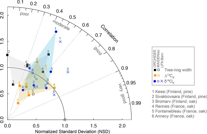
Although ORCHIDEE is able to simulate about 10 %– isotopic composition of source water (δ 18 Osw ) and leaf water
64 % (r = 0.31–0.80) of the observed 113 CR variability, it enrichment (118 Olw = δ 18 Olw −δ 18 Osw ) to simulated δ 18 OR
tends to underestimate its amplitude by 30 %–60 %, particu- variability in each model. In contrast to LPX-Bern, OR-
larly in the northernmost sites of pine (Kessi and Sivakko- CHIDEE simulates a much stronger contribution of δ 18 Osw
vaara) where the isotopic ratios were measured over the (46 %–85 %) than 118 Olw (14 %–53 %) to δ 18 OR variabil-
whole ring (Fig. 2). With the exception of the northern- ity (Fig. 3a). The δ 18 OR variability simulated by LPX-Bern
most site, the amplitude of δ 18 OR variability is simulated is dominated by the 118 Olw (42 %–78 %) isotopic signal
within ± 20 % and the simulations account for 13 %–55 % (Fig. 3b). ORCHIDEE does not simulate any clear latitudi-
(r = 0.36–0.74) of the variance of the observations, with all nal pattern for the relative importance of δ 18 Osw and 118 Olw .
the sites falling in the region of moderate to good perfor- In contrast, LPX-Bern simulates an increasing importance of
mance in Fig. 2. 118 Olw toward the north, except at the coolest northernmost
The δ 18 OR simulations of the LPX-Bern global model are site where δ 18 OR is dominated by the signature of δ 18 Osw in
systematically better than the simulations of ORCHIDEE the two models.
Biogeosciences, 18, 3781–3803, 2021 https://doi.org/10.5194/bg-18-3781-2021J. Barichivich et al.: Tree rings in ORCHIDEE 3791 Figure 3. Drivers of simulated δ 18 OR variability and consistency between isotopic forcings and simulations of ORCHIDEE and LPX-Bern across the climate gradient from boreal Finland (left) to temperate France (right). (a) Simulated contributions of source water (δ 18 Osw ; turquoise) and leaf water enrichment (118 Olw ; green) signals to δ 18 OR variability during 1960–2000. The percentage of explained variance (r 2 ) is indicated in each bar. (b) Correlation between the isotopic composition of precipitation (δ 18 Op ; light gray) and air vapor (δ 18 Ov ; dark gray) used to force the models and the resulting δ 18 Osw (turquoise), 118 Olw (green), and δ 18 OR (dark blue) simulated by ORCHIDEE and LPX-Bern during 1960–2000. All variables were averaged over the period May–August. Significance at the 95 % confidence level is indicated by the black dots. The isotopic signatures of precipitation (δ 18 Op ) and va- Taken together, the analysis of the isotopic forcings and con- por (δ 18 Ov ) from the LMDz atmospheric model used to tributions of source water and leaf enrichment suggests that drive ORCHIDEE are poorly correlated with those produced the better performance of LPX-Bern derives from the higher by the ECHAM5 atmospheric model that underlay δ 18 Osw contribution of leaf enrichment to simulated δ 18 OR variabil- used to force LPX-Bern (Fig. 3c). In spite of this lack ity. of agreement, the soil-integrated δ 18 Osw variability simu- ORCHIDEE overestimates the correlation between δ 18 OR lated by ORCHIDEE and JSBACH (coupled with ECHAM5) and 113 CR in the temperate sites in France, but it simulates land surface models is significantly correlated. The strength the magnitude of the isotopic coupling observed in the bo- of the correlations increases for the resulting 118 Olw and real oak and pine sites in Finland very well (Fig. 4a). This δ 18 OR variability simulated by ORCHIDEE and LPX-Bern means that the simulated stomatal control and responses to (Fig. 3c). This pattern of correlations indicates that, in mod- atmospheric humidity are overestimated in the temperate de- els, seasonal differences in the isotopic composition of pre- ciduous PFT, as is apparent in a stronger correlation between cipitation are strongly buffered by water mixing in the soil simulated isotopic ratios and VPD in these sites compared profile, resulting in coherent isotopic variations in source wa- with the observations (Fig. 4b–c). ter and thereby contributing to the correlation of the δ 18 OR Measured latewood or whole-ring isotopic ratios have no signals simulated by the models. The significant resemblance significant first-order autocorrelation in the sites (Fig. 5b– of simulated 118 Olw between the models points to simi- c), with the exception of 113 CR in Fontainebleau. However, larities in the response of leaf evaporative enrichment and ORCHIDEE simulates substantial autocorrelation in δ 18 OR meteorological forcings (i.e., vapor pressure deficit, VPD). variability in the three temperate sites in France and also in https://doi.org/10.5194/bg-18-3781-2021 Biogeosciences, 18, 3781–3803, 2021
3792                                                                                 J. Barichivich et al.: Tree rings in ORCHIDEE

                                                                         Figure 5. First-order autocorrelation in observed (black) and simu-
                                                                         lated (gray) tree-ring variables over the period 1960–2000. (a) Tree-
Figure 4. Observed and simulated isotopic coupling and response to       ring width. (b) 113 CR . (c) δ 18 OR . For Annecy the period of analy-
VPD across the climate gradient during 1960–2000. (a) Correlation        sis is 1971–2000. Significance at the 95 % confidence level is indi-
between δ 18 OR and 113 CR in simulations (gray) and observations        cated by the black dots.
(black). (b–c) Correlations between growing season VPD and sim-
ulated (gray) and observed (black) δ 18 OR and 113 CR variability,
respectively. For Annecy the period of analysis is 1971–2000. Sig-
nificance at the 95 % confidence level is indicated by the black dots.   4     Discussion

                                                                         4.1    Uncertainties and critical processes for modeling
                                                                                tree-ring width and isotopic ratios in a global model
the northernmost boreal site in Finland (Fig. 5c), likely as a
result of autocorrelation in the isotopic composition of source          Our evaluation in Fontainebleau and the other five sites
water. In contrast, simulated 113 CR has significant autocor-            across a boreal-to-temperate climate gradient in Europe
relation only in Rennes, although it is nearly significant as            showed that ORCHIDEE better simulates the interannual
well in Fontainebleau (Fig. 5b).                                         variability of tree-ring stable isotopes than ring width (30 %–
                                                                         64 % and < 30 % of the observed variability, respectively),
3.3    Simulated relationship between productivity and                   with a general performance for the stable isotopes similar
       isotopic variability                                              to MAIDENiso and slightly lower than LPX-Bern (Figs. 1
                                                                         and 2). The lower skill for tree-ring width results primar-
Growing season (May–August) GPP is significantly corre-                  ily from the inability of ORCHIDEE to simulate the signif-
lated with the simulated isotopic variability across all sites           icant temporal autocorrelation observed in ring width vari-
(Fig. 6a). The relationship is more consistent with δ 18 OR              ability (Fig. 6a). Temporal carryover is characteristic of tree-
(r = −0.47 to −0.73) than with 113 CR (r = −0.40 to 0.85)                ring width (Fritts, 1976; Cook, 1985) and varies consider-
along the climate gradient. The strength of the correlations             ably with species and location, accounting for 20 %–25 %
between δ 18 OR and GPP (r = −0.47 to −0.73) appears to                  of current-year ring width variability (Breitenmoser et al.,
increase from the boreal to the temperate region. This em-               2014). Several developmental and physiological processes
pirical relationship is driven by a synergistic effect of source         involved in tree growth can produce carryover, including pri-
water and leaf water enrichment because both variables cor-              marily remobilization of non-structural carbohydrates from
relate negatively with GPP (Fig. 6b). Leaf water enrichment              previous years (Kagawa et al., 2006; Keel et al., 2006; Car-
tends to correlate with GPP more strongly than source wa-                bone et al., 2013), cambial dynamics (Vaganov et al., 2011),
ter, though in the northernmost pine site only source water is           leaf lifespan (LaMarche and Stockton, 1974; Monserud and
correlated with GPP. Simulated tree-ring width is highly cor-            Marshall, 2001), and environmental cycles or slowly vary-
related with simulated GPP because of its direct dependency              ing crown and root dynamics that affect tree water and car-
on it (Fig. 6a).                                                         bon balance across several years (Fritts, 1976; Rocha et al.,

Biogeosciences, 18, 3781–3803, 2021                                                          https://doi.org/10.5194/bg-18-3781-2021
You can also read