A2A: 21,000 bulge stars from the ARGOS survey with stellar parameters on the APOGEE scale
←
→
Page content transcription
If your browser does not render page correctly, please read the page content below
Astronomy & Astrophysics manuscript no. aanda                                                                                       ©ESO 2021
                                               June 29, 2021

                                                         A2A: 21,000 bulge stars from the ARGOS survey with stellar
                                                                     parameters on the APOGEE scale
                                                    S.M. Wylie1       ?,   O.E. Gerhard1      , M.K. Ness2, 3      , J.P. Clarke1     , K.C. Freeman4, 6 , and J. Bland-Hawthorn5, 6

                                                     1
                                                         Max-Planck-Institut fur Extraterrestrische Physik, Gießenbachstraße, D-85748 Garching, Germany
                                                     2
                                                         Department of Astronomy, Columbia University, Pupin Physics Laboratories, New York, NY 10027, USA
                                                     3
                                                         Center for Computational Astrophysics, Flatiron Institute, 162 Fifth Avenue, New York, NY 10010, USA
                                                     4
                                                         Research School of Astronomy & Astrophysics, Australian National University, ACT 2611, Australia
                                                     5
                                                         Sydney Institute for Astronomy, School of Physics, A28, The University of Sydney, NSW 2006, Australia
                                                     6
                                                         Centre of Excellence for All-Sky Astrophysics in Three Dimensions (ASTRO 3D), Australia
arXiv:2106.14298v1 [astro-ph.GA] 27 Jun 2021

                                                     Received-; accepted -

                                                                                                                 ABSTRACT

                                                     Aims. Spectroscopic surveys have by now collectively observed tens of thousands of stars in the bulge of our Galaxy. However, each
                                                     of these surveys had unique observing and data processing strategies which led to distinct stellar parameter and abundance scales.
                                                     Because of this, stellar samples from different surveys cannot be directly combined.
                                                     Methods. Here we use the data-driven method, The Cannon, to bring 21,000 stars from the argos bulge survey, including 10,000 red
                                                     clump stars, onto the parameter and abundance scales of the cross-Galactic survey, apogee, obtaining rms precisions of 0.10 dex, 0.07
                                                     dex, 74 K, and 0.18 dex for [Fe/H], [Mg/Fe], Teff , and log(g), respectively. The re-calibrated argos survey - which we refer to as the
                                                     a2a survey - is combined with the APOGEE survey to investigate the abundance structure of the Galactic bulge.
                                                     Results. We find X-shaped [Fe/H] and [Mg/Fe] distributions in the bulge that are more pinched than the bulge density, a signature
                                                     of its disk origin. The mean abundance along the major axis of the bar varies such that the stars are more [Fe/H]-poor and [Mg/Fe]-
                                                     rich near the Galactic center than in the long bar/outer bulge region. The vertical [Fe/H] and [Mg/Fe] gradients vary between the
                                                     inner bulge and long bar with the inner bulge showing a flattening near the plane that is absent in the long bar. The [Fe/H]-[Mg/Fe]
                                                     distribution shows two main maxima, an “[Fe/H]-poor [Mg/Fe]- rich” maximum and an “[Fe/H]-rich [Mg/Fe]-poor” maximum, that
                                                     vary in strength with position in the bulge. In particular, the outer long bar close to the Galactic plane is dominated by super-solar
                                                     [Fe/H], [Mg/Fe]-normal stars. Stars composing the [Fe/H]-rich maximum show little kinematic dependence on [Fe/H], but for lower
                                                     [Fe/H] the rotation and dispersion of the bulge increase slowly. Stars with [Fe/H] < −1 dex have a very different kinematic structure
                                                     than stars with higher [Fe/H].
                                                     Conclusions. Comparing with recent models for the Galactic boxy-peanut bulge, the abundance gradients and distribution, and the
                                                     relation between [Fe/H] and kinematics suggest that the stars comprising each maximum have separate disk origins with the “[Fe/H]-
                                                     poor [Mg/Fe]-rich” stars originating from a thicker disk than the “[Fe/H]-rich [Mg/Fe]-poor” stars.
                                                     Key words. Stars: abundances, fundamental parameters; Galaxy: abundances, bulge, formation; Methods: data analysis

                                               1. Introduction                                                            bulge has been found to contain stars that are part of the bar,
                                                                                                                          inner thin and thick disks, and a pressure supported component
                                               The Milky Way bulge is notoriously difficult and expensive to              (Queiroz et al. 2020b). Furthermore, there is evidence that the
                                               observe due to the high extinction along our sightline to the              bulge also contains a remnant of a past accretion event, the in-
                                               Galactic Centre. Nevertheless, over the past two decades, the              ner Galaxy structure (Horta et al. 2021). Multiple age studies of
                                               number of spectroscopically observed bulge stars has increased             the bulge have reported that while the bulge is mainly composed
                                               from a few hundred to tens of thousands thanks to multiple spec-           of old stars (∼10 Gyr), it contains a non-negligible fraction of
                                               troscopic stellar surveys such as argos (Freeman et al. 2012),             younger stars (Bensby et al. 2013, 2017; Schultheis et al. 2017;
                                               Gaia-eso (Gilmore et al. 2012), GIBS (Zoccali et al. 2014),                Bovy et al. 2019; Hasselquist et al. 2020).
                                               apogee (Majewski 2016), and Gaia (Cropper et al. 2018).                        While analysis of these surveys has greatly improved our un-
                                                   The extensive coverage of these spectroscopic surveys has              derstanding of the bulge, direct comparisons of studies that use
                                               led to many novel discoveries and vastly improved our under-               different survey data, as well as combinations of the measure-
                                               standing of bulge formation and evolution. We know from its                ments of the stars from different survey pipelines is problematic.
                                               wide, multi-peaked metallicity distribution function (MDF) that            This is because different surveys use different selection criteria,
                                               the bulge is composed of a mixture of stellar populations. This is         wavelength coverage, and spectral resolution. Furthermore, they
                                               further supported by the different populations, defined by their           employ different data analysis methods, assume different under-
                                               metallicities, exhibiting different kinematics (Hill et al. 2011;          lying stellar models, and make different approximations to derive
                                               Ness et al. 2013b; Rojas-Arriagada et al. 2014, 2017; Zoccali              stellar parameters and individual element abundances from their
                                               et al. 2017). Through careful chemodynamical dissection, the               spectra (see Jofré et al. (2019) for a review).
                                                                                                                              Despite these inconsistencies, analyses that employ stars
                                                ?
                                                    swylie@mpe.mpg.de                                                     from different surveys are often compared, leading to uncertainty
                                                                                                                                                                     Article number, page 1 of 26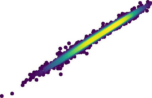
A&A proofs: manuscript no. aanda

                                                                                      15
as to whether the results reflect intrinsic properties of the Galaxy
or if they are simply due to different observing and data pro-                        10
cessing strategies. For example, Zoccali et al. (2017) and Rojas-
Arriagada et al. (2017) found bi-modal bulge MDFs using data                           5
from the Gaia-eso and GIBS surveys, Rojas-Arriagada et al.

                                                                           b (deg)
(2020) found a three component bulge MDF using data from the                           0
apogee survey, and Ness et al. (2013a) found a five component
bulge MDF using data from the argos survey. Because the stars                        −5
in these surveys have not been observed and analyzed in the ex-
act same manner, it is unclear whether these differences in the                      −10
bulge MDF arise because of different parameter and abundance
scales or because of different selection functions.                                  −15
                                                                                       −40   −20           0          20          40
    In this paper, we use the data driven method, The Cannon
                                                                                                        l (deg)
(Ness et al. 2015), to put 21,000 stars from the Galactic bulge
survey argos onto the parameter and abundance scales of the            Fig. 1. Locations of the apogee (blue ellipses and red crosses) and argos
cross-Galactic survey apogee. Of these 21,000 stars, there are         (green ellipses) bulge fields. The red crosses indicate apogee fields that
roughly 10,000 red clump (RC) stars with accurate distances.           either have no or poor survey selection function estimates. The marker
By rectifying the scale differences between the two surveys, we        size indicates the field size.
can combine them and gain a deeper coverage of the Galactic
bulge. We call the re-calibrated argos catalog the a2a catalog
as we are putting argos stars onto the apogee scale. Then, using       from the stellar colours (J − Ks )0 using the calibration by Bessell
the combined a2a and apogee surveys, we investigate the chemo-         et al. (1998). For more information about the argos parameter
dynamical structure of the bulge. Specifically, we examine how         and abundance determination process see Freeman et al. (2012).
the Iron abundance and Magnesium enhancement vary over the                 The argos catalog used in this paper contains 25, 712
bulge as well as their kinematic dependencies.                         stars/spectra from the original 28, 000 observed. The missing
    The paper is structured as follows: In Section 2 we describe       stars/spectra were removed because they had low signal-to-noise
the argos and apogee surveys as well as highlight the incon-           (SNR) and poor quality spectra (Freeman et al. 2012). The num-
sistencies between them which make directly combining them             ber of pixels of each argos flux array is 1697. To process the
questionable. In Section 3 we summarize the technical back-            data, we re-normalized the remaining argos spectra by divid-
ground of The Cannon. In Section 4 we explain how we apply             ing each by a Gaussian-smoothed version of itself, with the
The Cannon to the argos catalog to create the a2a catalog. In          Calcium-triplet lines removed, using a smoothing kernel of 10
Section 4 we also describe the three validation tests we perform       nm. We also transformed each spectrum to a common rest frame
to verify that the label transfer was successful. In Section 5 we      and masked out the diffuse interstellar band at 8621 nm. We also
discuss the selection functions of the a2a and apogee surveys.         masked out the region around 8429 nm as we found that this re-
In Section 6 we use the a2a and apogee catalogs to examine the         gion had a strong residual between the mean spectra of positive
abundance structure of the Galactic bulge. In Section 7 we dis-        and negative velocity stars, indicating that it is systematically
cuss the results of the paper in more detail and finally in Section    affected by the velocity shift.
8 we end the paper with our conclusions.
                                                                       2.2. APOGEE

2. Data                                                                The Apache Point Observatory Galactic Evolution Experiments
                                                                       (apogee; Majewski (2016)) is a program in the Sloan Digital
In this section, we provide some background on the data used in        Sky Survey (SDSS) that was designed to obtain high resolution
this paper before discussing their main properties.                    spectra of red giant stars located in all major components of the
                                                                       Galaxy. The survey operates two telescopes ; one in each hemi-
2.1. ARGOS                                                             sphere with identical spectrographs which observe in the near-
                                                                       infrared between 1.5µm to 1.7µm at a resolution of R ' 22, 500.
The Abundance and Radial Velocity Galactic Origin Survey               In this work, we use the latest data release, DR16 (Ahumada
(argos; Freeman et al. (2012); Ness et al. (2013a,b)) is a medium      et al. 2019), which is the first data release to contain stars ob-
resolution spectroscopic survey designed to observe RC stars           served in the southern hemisphere. The locations of the apogee
in the Galactic bulge. Using the AAOmega fibre spectrometer            fields used in this work are shown in Figure 1 as blue ellipses
on the Anglo-Australian Telescope, ARGOS observed nearly               and red crosses.
28, 000 stars located in 28 fields directed towards the bulge. The         Stellar parameters and abundances of the apogee stars used
field locations are shown as green ellipses in Figure 1. The obser-    in this work were obtained from the apogee Stellar Parame-
vations were performed across a wavelength region of 840−885           ters and Chemical Abundance Pipeline (ASPCAP; García Pérez
nm at a resolution of R = λ/δλ ' 11, 000, where δλ is the spec-        et al. (2016); Holtzman et al. (2018); Jönsson et al. (2020)).
tral resolution element.                                               This pipeline uses the radiative transfer code Turbospectrum
     The argos team determined the Iron abundance ([Fe/H]),            (Plez et al. 1992; Plez 2012) to build a grid of synthetic spectra.
surface gravity (log(g)), and alpha enhancement ([α/Fe]) of each       The parameters and abundances were determined using the code
star in their catalog using χ2 minimisation to find the best fit be-   FERRE (Allende Prieto et al. 2006) which iteratively calculates
tween the observed spectra and a library of synthetic spectra.         the best-fit between the synthetic and observed spectra. The fun-
The Local Thermodynamic Equilibrium stellar synthesis pro-             damental atmospheric parameters such as log(g), Teff , and over-
gram MOOG (Sneden et al. 2012) was used to generate the li-            all metallicity were determined by fitting the entire apogee spec-
brary of spectra. The effective temperature (Teff ) was determined     trum of a star. Individual elemental abundances were determined
Article number, page 2 of 26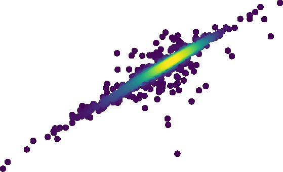
S.M. Wylie      et al.: A2A: 21,000 bulge stars from the ARGOS survey with stellar parameters on the APOGEE scale

by fitting spectral windows within which the spectral features of                                            0.5
                                                                                                                      bias: -0.02

                                                                          ARGOS [Fe/H] (dex)
a given element are dominant.                                                                                         rms: 0.22
                                                                                                             0.0
    We obtain spectrophotometric distances for the apogee stars
from the AstroNN catalog (Leung & Bovy 2019; Mackereth                                              −0.5
et al. 2019a), which derives them from a deep neural network
trained on stars common to both apogee and Gaia (Gaia Collab-                                       −1.0
oration et al. 2018).
                                                                                                    −1.5
    In this work, we specifically focus on apogee stars located in
fields directed towards the bulge with |lf | < 35° and |bf | < 13°                                  −2.0
where lf and bf are the Galactic longitude and latitude loca-                                          −2.0               −1.5       −1.0      −0.5         0.0          0.5
tions of the fields. We remove 6 fields that were designed to ob-                                                                APOGEE [Fe/H] (dex)
serve the core of Sagittarius. We require that the stars are part                                            0.6
of the apogee main sample (MSp) by setting the apogee flag,                                                           bias: 0.07

                                                                          ARGOS [α/Fe] (dex)
                                                                                                                      rms: 0.12
EXTRATARG, to zero. We refer to this sample as the apogee
                                                                                                             0.4
bulge MSp. To ensure that the stars we use have trustworthy pa-
rameters and abundances, we also require the stars to have valid
                                                                                                             0.2
ASPCAP parameters and abundances, SNR ≥ 60, Teff ≥ 3200
K, and no Star_Bad flag set (23rd bit of ASPCAPFLAG = 0).
After applying these cuts, there are 172 remaining bulge fields                                              0.0
containing 37, 313 stars. For reference, we refer to this sample
as the HQ apogee bulge MSp.                                                                         −0.2
                                                                                                                         0.0                0.2                   0.4
    In the analysis sections of this work, unless explicitly stated
otherwise, we further restrict our apogee sample to only stars                                                                 APOGEE [Mg/Fe] (dex)
for which we can obtain good selection function estimates. This
sample contains 23, 512 stars and we refer to it as the HQSSF                                         5500            bias: 285
                                                                                                                      rms: 321
apogee bulge MSp. See Section 5.2 for further details on this
                                                                          ARGOS Teff (K)

sample.
                                                                                                      5000

2.3. Survey Inconsistencies
                                                                                                      4500
After the removal of potential binaries though visual inspection
of individual spectra, we find 204 stars that are observed by both
the apogee and argos surveys. Using these stars we can deter-                                         4000
                                                                                                                        4000                4500                  5000
mine whether the surveys are consistent by checking that they                                                                       APOGEE Teff (K)
derive the same parameters and abundances for the same stars.
    In Figure 2, we compare the [Fe/H], α-enhancements, Teff ,                                               3.5
                                                                                                                      bias: 0.30
and log(g) of the common stars. The argos α-enhancement is
                                                                                        ARGOS log(g) (dex)

                                                                                                                      rms: 0.47
the average of the individual α-elements over Iron ([α/Fe]). For                                             3.0

apogee stars, ASPCAP provides individual α-elements with re-
                                                                                                             2.5
spect to Iron ([Mg/Fe], [O/Fe], [Ca/Fe], ...) as well as an av-
erage of the α-elements to metallicity ([α/M]). For our com-                                                 2.0
parisons, we choose the ASPCAP Magnesium enhancement
([Mg/Fe]) because Magnesium is produced only by SN-II with                                                   1.5
no contribution from SN-Ia. The bias and rms of each distribu-
tion are given in the upper left hand corner of each plot. The bias                                          1.0
                                                                                                                1.0        1.5        2.0          2.5        3.0         3.5
is calculated by subtracting the apogee values from the argos                                                                    APOGEE log(g) (dex)
values and taking the mean of the differences.
    The [Fe/H] comparison in the first plot of Figure 2 shows          Fig. 2. apogee derived parameters (x-axis) versus argos derived param-
that the surveys roughly agree between ∼ − 0.75 dex and ∼0             eters (y-axis) for the 204 reference set stars observed by both surveys.
dex (limits in apogee [Fe/H]) with a scatter of ∼0.16 dex.             The bias (mean of the differences) and rms of the distributions are given
However, beyond these limits, the deviation between the sur-           in the upper left hand corner of each plot. The reference set stars that are
                                                                       within one argos observational error, 0.13 dex (0.1 dex), from the max-
veys increases, reaching up to ∼0.4 dex. The α-enhancement             imum [Fe/H] ([α/Fe]) value reached by the reference set are plotted as
Magnesium-enhancement comparison in the second plot shows              blue crosses (red triangles).
that the argos [α/Fe] estimates are on average ∼0.07 dex larger
than the apogee [Mg/Fe] estimates. If we instead compare the
argos [α/Fe] estimates to the apogee [α/Fe] estimates then the
bias and rms of the distribution are larger at 0.12 dex and 0.15
dex respectively. The Teff comparison in the third plot shows that     This could be due to a number of factors such as observing in dif-
the argos Teff estimates are on average ∼300 K hotter than the         ferent wavelength regions (e.g. optical in argos versus infrared
apogee Teff estimates. Finally, while there is a lot of scatter, the   in apogee), their use of different data analysis methods (e.g. pho-
log(g) comparison in the last plot shows that the argos log(g)         tometric temperatures in argos versus spectroscopic tempera-
values are generally higher than the apogee log(g) values.             tures in apogee), or their use of different stellar models. In the
    The parameter comparisons show that for most of the com-           following sections, we use the data driven method, The Cannon,
mon stars, the apogee and argos parameters differ significantly.       and this set of common stars to bring the apogee and argos sur-
                                                                                                                                                         Article number, page 3 of 26
A&A proofs: manuscript no. aanda
veys on to the same parameter and abundance scales, thereby Here the label matrix, ln , is quadratic in the labels and for
correcting the deviations we see in Figure 2. each star (each column in the matrix) has the form:
ln ≡ [1, l(1...n) , l(1...n) · l(1...n) ]. (2)
3. The Cannon Method
The Cannon is a data-driven method that can cross-calibrate If, for example, the generative model is trained on the labels Teff
spectroscopic surveys. It has the advantage that it is very fast, and log(g), then each column in the label matrix would be:
requires no direct spectral model, and has measurement accu-
ln ≡ [1, Teff , log(g), Teff · Teff , log(g) · log(g), Teff · log(g)] (3)
racy comparable to physics based methods even at lower SNR.
The Cannon has been previously used to put different surveys on
The noise, σ, is the rms combination of the uncertainty in the
the same parameter and abundance scales using common stars
flux at each wavelength due to observational errors, σnλ , and the
(Casey et al. 2017; Ho et al. 2017; Birky et al. 2020; Galgano
intrinsic scatter at each wavelength in the model, sλ .
et al. 2020; Wheeler et al. 2020).
The Cannon uses a set of reference objects with known labels Equation 1 corresponds to the single-pixel log-likelihood
(i.e. Teff , log(g), [Fe/H], [X/Fe] ...), that well describe the spec- function:
tral variability, to build a model to predict the spectrum from the 1 [ fnλ − θλT · ln ]2 1
labels. This model is then used to re-label the remaining stars in ln p( fnλ |θλT , ln , sλ ) = − − ln(s2λ + σ2nλ ). (4)
the survey. The word "label" is a machine learning term that we 2 s2λ + σ2nλ 2
use here to refer to stellar parameters and abundances together
with one term. The set of common stars used to build the model During the training step, the coefficient matrix θλ and the model
is called the reference set. scatter sλ are determined by optimising the single-pixel log-
The Cannon is built on two main assumptions: likelihood in Equation 4 for every pixel separately:
1. Stars with the same set of labels have the same spectra. N
X stars
2. Spectra vary smoothly with changing labels. θλ , sλ ← argmax ln p( fnλ |θλT , ln , sλ ). (5)
θλ ,sλ n=1
Consider two surveys, A and B, where we want to put
the stars in survey A onto the label scales of survey B using During this step The Cannon uses the reference set stars to pro-
The Cannon. Assume we also have the required set of common vide the label matrix, ln . The label matrix is held fixed while the
stars between the two surveys to form the reference set. To cross coefficient matrix and model scatter are treated as free parame-
calibrate the surveys, The Cannon performs two main steps: the ters.
training step and the application step. During the training step,
the spectra from survey A and the labels from survey B of the ref-
erence set stars are used to train a generative model. Then, given 3.2. The Application Step
a set of labels, this model predicts the probability density func- In the training step, we have the label matrix, ln , and we solve
tion for the flux at each wavelength/pixel. During the application for the coefficient matrix θλ and the scatter sλ . In the applica-
step, the spectra of a new set of survey A stars (not the reference tion step, we do the opposite: we have the coefficient matrix θλ
set) are relabeled by the trained model. We call this set of stars and the scatter sλ and we solve for a new label matrix, lm . The
the application set. If the region of the spectra fit to carries the subscript m is used in this step because the label matrix now cor-
label information and the reference set well represents the ap- responds to stars in the application set, not the reference set.
plication set, then the new labels of survey A’s stars should be The label matrix, lm , is solved for by optimising the same
on survey B’s label scales. The success of the re-calibration can log-likelihood function as Equation 4. However, here this opti-
be quantified with a cross-validation procedure, the pick-on-out misation is performed using a non-linear least squares fit over
test described in Section 4.2, which returns the systematic uncer- the whole spectrum, instead of per pixel:
tainty with which labels can be inferred from the data, as well as
a comparison of the generated model spectra to the observational Npix
spectra for individual stars, using a χ2 metric.
X
lm ← argmax ln p( fmλ |θλT , lm , sλ ). (6)
In the next two subsections, we will describe the main steps lm λ=1
of The Cannon in more detail.
4. A2A Catalog
3.1. The Training Step
In this paper, we use The Cannon to put the stars from the argos
During the training step, a generative model is trained such that survey onto the apogee survey’s label scales for the following la-
it takes the labels as input and returns the flux at each wave- bels: [Fe/H], [Mg/Fe], Teff , log(g), and K-band extinction (Ak ).
length/pixel of the spectrum. The functional form of the genera- After applying The Cannon to the argos survey, we obtain a new
tive model, fnλ , can be written as a matrix equation: catalog containing the same stars observed by the argos survey
fnλ = θλT · ln + σ, (1) but with new label values. Other labels, such as line-of-sight ve-
locity or apparent magnitude, remain unchanged. We call this
where θλ is a coefficient matrix, ln is a label matrix, and σ is new catalog the a2a catalog. In this Section, we describe the ref-
the noise. The subscript n indicates the reference set star while erence and application sets used to build the a2a catalog and
subscript λ indicates the wavelength/pixel. perform three validation tests to confirm that the a2a catalog is
The coefficient matrix, θλ , contains the coefficients that con- on the apogee scale. Lastly, we compare the a2a catalog to the
trol how much each label affects the flux at each pixel. The co- argos catalog and explain how we extract the a2a RC and corre-
efficients are calculated during the training step. sponding distances.
Article number, page 4 of 26S.M. Wylie et al.: A2A: 21,000 bulge stars from the ARGOS survey with stellar parameters on the APOGEE scale
30 all the limits by 1σARG , equal to the argos observational error
Fe-m1σ [Fe/H] (dex)
0.50 bias: -0.01
rms: 0.03 of each label, then we would include 2704 more stars in the ap-
0.25
20
plication set (∼10.5% more of the argos catalog). Because these
stars are still close to the reference set stars, the labels returned
N
0.00
by The Cannon for these stars may be correct to the first order.
−0.25 10 To test whether we can extend any of the limits we use the fol-
−0.50 lowing procedure:
−0.50 −0.25 0.00 0.25 0.50 1. Remove reference set stars 1σARG from each limit. This de-
Original [Fe/H] (dex) creases the number of reference set stars.
0.5 2. Train a new Cannon model on the reduced reference set. For
Mg-m1σ [Mg/Fe] (dex)
bias: 0.00 300 clarity, we refer to this model as the minus-one-sigma (m1σ)
0.4 rms: 0.02 model.
0.3 200 3. Reprocess argos spectra using the m1σ model to obtain new
Cannon parameters for each star. The application set remains
N
0.2 the same as the one processed by the original Cannon model.
100 4. Compare the new Cannon labels from the m1σ model to the
0.1
labels given by the original Cannon model.
0.0
0.0 0.1 0.2 0.3 0.4 0.5 For reference, the argos observational errors, σARG , for [Fe/H],
Original [Mg/Fe] (dex) [α/Fe], Teff , and log(g) are: 0.13 dex, 0.1 dex, 100 K, and 0.3
dex respectively.
Fig. 3. Comparison of the [Fe/H] (top) and [Mg/Fe] (bottom) labels
We applied this test to each label limit separately and found
generated by the original Cannon model (x-axis) and the m1σ models
(y-axis). In the top plot, only stars with argos 0.05 < [Fe/H] (dex) < that the extrapolation works best for the high [Fe/H] and high
0.18 are compared (the region in [Fe/H] spanned by the blue crosses in [α/Fe] limits. In Figure 3, we compare the output labels pro-
the top plot of Figure 2). In the bottom plot, only stars with argos 0.47 < duced by the original Cannon model against the output labels
[α/Fe] (dex) < 0.57 are compared (the region in [α/Fe] spanned by the produced by the m1σ models trained on the reduced reference
red triangles in the plot second from the top in Figure 2). The points are sets. The original Cannon model was trained on all 204 reference
coloured by the point density.The black lines are one-to-one lines and set stars, shown as the black, blue, and red markers in Figure 2.
blue lines indicate ±1σARG . The bias and rms of each distribution are The Fe-m1σ model (top plot) was trained on 149 reference set
given in the top left corner of each plot. stars, shown as just the black and red markers in Figure 2. The
Mg-m1σ model (second plot) was trained on 199 reference set
4.1. Reference and Application Sets stars, shown as just the black and blue markers in Figure 2. For
each comparison (or plot) we only compare stars that have argos
A reference set of stars, which is used to train The Cannon’s parameter values in the 1σARG region we removed (regions oc-
model, is comprised of the stars that are observed by both sur- cupied by the blue and red markers in Figure 2). For both la-
veys. The labels for this reference set come from the survey with bels, less than 1% of stars have original Cannon model and m1σ
the desired label scale (in our case apogee), while the spectra model labels that differ by more than 1σARG .
are taken from the other (in our case argos). The model that is We also compared the labels produced by the original
learned at training time should only be applied to stars that are Cannon model to the labels produced by a Cannon model that
well represented by the reference set. That is, applied to stars was trained on a reference set that was simultaneously reduced
that span the label region of the training data, within which the by 1σARG in [Fe/H] and [Mg/Fe]. The reference set of this
model can interpolate but need not extrapolate. This can also be model consists of only 144 stars, shown as the black markers
thought of as a selection in spectra. In our case, the 204 stars that in Figure 2. We find that less than 1% of stars from this model
are common to both the apogee and the argos surveys (discussed have labels that differ from the original Cannon model by more
in Section 2.3) form the reference set for our Cannon model. The than 1σARG in [Fe/H] and 2% in [Mg/Fe].
average SNR of the reference set is 46 for argos and 107 for Because we find that we can accurately predict the [Fe/H]
apogee. and [Mg/Fe] labels of stars in the 1σARG regions of the parame-
These reference set stars are found in the following intervals ter space removed from the reference set, we make the assump-
in the argos parameter space: tion that we can apply the Cannon model trained on all 204 ref-
4195 ≤ Teff (K) ≤ 5444 (7a) erence set stars to stars with argos parameters 1σARG beyond the
high [Fe/H] and [α/Fe] limits and still get approximately correct
1.393 ≤ log(g) (dex) ≤ 3.376 (7b) labels. Thus, we extend the limits of 7c and 7d to be:
−1.4 ≤ [Fe/H] (dex) ≤ 0.18 (7c)
−1.4 ≤ [Fe/H] (dex) ≤ 0.31 (8a)
−0.062 ≤ [α/Fe] (dex) ≤ 0.569 (7d)
−0.062 ≤ [α/Fe] (dex) ≤ 0.669 (8b)
We ignore the limits in Ak as this label was only included to
stabilize the fits to the other labels. As such, we do not use the Limits 7a,7b, 8a, and 8b enable us to process 85% of the argos
learned Ak label for science. catalog, or 21, 577 stars. This increases the number of stars in
There are 20,435 argos stars (∼79% of the argos catalog) the a2a catalog with [Fe/H] above 0.5 dex by roughly 45%,
within the 4D parameter space defined by intervals 7a to 7d. the number of stars with [Fe/H] between 0 dex and 0.5 dex by
These stars are considered to be well represented by the refer- roughly 23%, and the stars with [Fe/H] below −1 dex by roughly
ence set and normally would form our application set. However, 10%.
there are many stars with parameter values close to but just out- In Section 5.1.2, we define our a2a catalog used for the bulge
side of the reference set limits. For example, if we could extend analysis. This final catalog has an additional colour cut applied
Article number, page 5 of 26A&A proofs: manuscript no. aanda
CANNON [Fe/H] (dex)
0.5 bias: 0.00
3500
rms: 0.10
0.0
1500
−0.5
−1.0
N
1000
−1.5
−2.0 3000 500
−2.0 −1.5 −1.0 −0.5 0.0 0.5
APOGEE [Fe/H] (dex)
0
0.5 0 1000 2000 3000 4000 5000
CANNON [Mg/Fe] (dex)
bias: 0.00
0.4 rms: 0.06 χ2
0.3
Fig. 5. The model χ2 distribution of a2a stars. The dashed orange line
2500
0.2 gives the number of pixels in each a2a/argos spectrum.
0.1
0.0 4.2. Validation Tests
−0.1
−0.1 0.0 0.1 0.2 0.3 0.4 0.5
χ2
Given a reference set and an application set, The Cannon will al-
APOGEE [Mg/Fe] (dex) ways return new labels for the stars in the application set. How-
2000 ever, if one is not careful, the returned labels can have large er-
5000 bias: -8.87 rors. In this section, we perform three validation tests to verify
CANNON Teff (K)
rms: 70.35 that the labels returned by The Cannon are reasonable.
4750
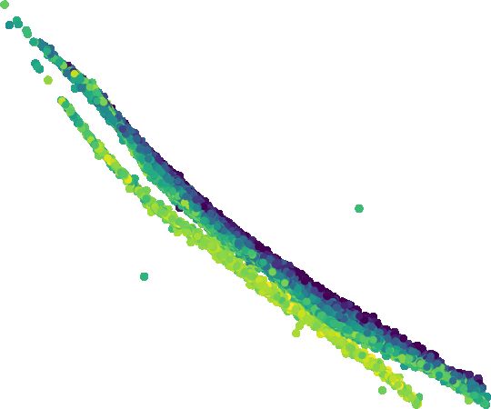
The first validation test we perform is a common machine
4500
learning test called the pick-one-out test. In this test, we create
204 models, each of which is trained on 203 stars from the ref-
4250 erence set. The single star that is left out from the reference set
1500 changes between each model. Every model is then applied to
4000 the spectra of the respective left out star to obtain a new set of
4000 4250 4500 4750 5000 labels for it. How similar the new set of labels are to the origi-
APOGEE Teff (K) nal apogee labels indicates how well The Cannon can learn the
apogee labels given the reference set. In Figure 4 we compare
CANNON log(g) (dex)
bias: -0.01 the new Cannon labels of these stars to their apogee labels. For
3.0 rms: 0.17 all four labels, the bias and rms, given in the upper left hand
1000
2.5
corner of each plot, are much lower than those from the argos-
apogee comparisons in Figure 2. The strong agreement indicates
2.0 that The Cannon can successfully learn the apogee labels from
the argos spectra using the reference set composed of the 204
1.5 common stars. The error on each parameter for each star in the
a2a catalog is calculated by adding in quadrature the rms value
1.0
1.0 1.5 2.0 2.5 3.0 from the pick-one-out test and the small error that is output by
APOGEE log(g) (dex) the optimiser of the The Cannon (see Section 3).
As a second validation test we compare the model and ob-
Fig. 4. Pick-one-out test. For each plot, each point represents a different
servational spectra. The shape of the spectrum of a star can be
reference set star. For a given point in a plot, the x-axis value is the
apogee derived label while the y-axis value is the label prediction from affected by many different stellar parameters and abundances.
a Cannon model trained on all other (203) reference set stars. Therefore, Ideally, when training a model to describe a stellar spectrum with
for each point in each plot the applied Cannon model is different than labels one would like to include all stellar labels that affect the
that of every other point. The points are coloured by their model χ2 spectrum’s shape. However, this would require a huge number of
values. The bias and rms of each distribution are given in the top left reference set stars, which we do not have. Instead, we are mak-
corner of each plot. ing the approximation that the argos spectra (8400 Å - 8800 Å)
can be well described by the five labels: [Fe/H], [Mg/Fe], Teff ,
log(g), and Ak . To test this, we compare the model spectra gener-
ated by The Cannon against the true observational spectra. This
can be done because The Cannon trained model returns the flux
(Equation 12) which removes an additional 252 stars leaving at each pixel when given the labels (Equation 1). In Figure 6
21, 325 stars in the final catalog. If the same colour cut is ap- we plot the argos spectra of a few example stars with a range
plied to the original argos catalog then the argos catalog would of [Fe/H] values and cumulative χ2 values (sum of the pixel
contain 23, 487 stars. The final colour cut a2a catalog is then χ2 values) around the argos pixel number (1697, see Figure 5)
91% complete compared to the colour cut argos catalog. The versus their model spectra generated by The Cannon. For the
parameter and abundance errors of the colour cut a2a catalog are model spectra, line thicknesses show the scatter of the fit by
calculated in Section 4.2. For [Fe/H], [Mg/Fe], Teff , and log(g), The Cannon at each wavelength. Figure 6 shows that the model
the rms of the errors, σA2A , are 0.10 dex, 0.07 dex, 74 K, and spectra closely reproduce the true observational spectra. The
0.18 dex respectively. overall good fit between the model spectra and the true spectra
Article number, page 6 of 26S.M. Wylie et al.: A2A: 21,000 bulge stars from the ARGOS survey with stellar parameters on the APOGEE scale
1.0
1.0
0.5
[Fe/H]: -0.49 dex
0.2
0.8
0.0
−0.2
8400 8450 8500 8550 8600 8650 8700 8750 8800
1.0
0.5
Normalized Flux
0.6 [Fe/H]: -0.26 dex
0.2
0.0
−0.2
1.0 8400 8450 8500 8550 8600 8650 8700 8750 8800
0.4
0.5
[Fe/H]: -0.03 dex
0.2
0.0 8400 8450 8500 8550 8600 8650 8700 8750 8800
−0.2
1.0 8400 8450 8500 8550 8600 8650 8700 8750 8800
0.2
0.5
[Fe/H]: 0.28 dex
0.2
0.0 8400 8450 8500 8550 8600 8650 8700 8750 8800
−0.2
0.0
8400 8450 8500 8550 8600 8650 8700 8750 8800
0.0 0.2 0.4 0.6 0.8 1.0
Wavelength λ(Å)
Fig. 6. The normalized argos spectra (black) versus the normalized model spectra (blue) generated by The Cannon for a2a stars with [Fe/H]
values between −0.5 . [Fe/H] . 0.25. The plotted line thicknesses of the model spectra indicate the scatter of each fit by The Cannon. The
residuals between the normalized argos spectra and normalized model spectra are also shown in the panels below the spectra.
0.0
0.5 though no isochrone information was input into The Cannon,
0.5 there are no a2a stars in nonphysical regions of the diagram. The
close fit of the a2a stars to the PARSEC isochrones supports that
1.0 0.0
the label transfer was successful.
[Fe/H] (dex)
log(g) (dex)
1.5
−0.5 The success of these three tests shows that it is possible to
2.0 train a Cannon model on a moderate number (204) of common
−1.0
stars and still obtain a set of labels with good precisions (see
2.5
Section 4.1).
3.0
−1.5
3.5
4.3. A2A versus ARGOS
4.0 −2.0
6000 4000 6000 4000
Teff (K) Teff (K) In this section we compare the a2a catalog to the argos cata-
Fig. 7. Teff -log(g) distribution of argos (left) and a2a (right) stars log. In Figure 7 we show the Teff -log(g)-[Fe/H] distributions of
coloured by mean [Fe/H]. 10Gyr PARSEC isochrones with −2 < argos stars (left) and a2a stars (right) on top of 10 Gyr PAR-
[Fe/H] (dex) < 0.6 are plotted beneath. Note, the isochrones are plotted SEC isochrones. The argos stars very roughly follow the PAR-
at 35% transparency in order to visually differentiate them from the 2D SEC isochrones. Many argos stars also fall in nonphysical re-
histograms. gions of the parameter space. As discussed in the previous sec-
tion, a2a stars have a much tighter alignment with the PARSEC
isochrones with no stars falling in nonphysical regions.
indicates that the spectra of the argos stars can be well described
by the variation of the five labels. In Figure 8 we show the argos and a2a MDFs of all stars
The third test we do is comparing the Teff -log(g)-[Fe/H] dis- (top) and only RC stars (bottom). The most prominent difference
tribution of a2a stars to theoretical distributions. In the right hand between the MDFs of the surveys is that a2a obtains more very
plot of Figure 7, we show the Teff -log(g) distribution of a2a stars [Fe/H]-rich stars than argos for all stars as well as when we
coloured by mean [Fe/H] on top of 10 Gyr PARSEC isochrones restrict to only the RC. argos has more solar to sub-solar stars
with metallicities ranging from −2 dex to 0.6 dex (Tang et al. until ∼ − 0.5 dex where a2a has more stars. Between ∼ − 1 and
2014; Chen et al. 2014, 2015; Bressan et al. 2012). The a2a ∼ − 0.7 dex argos has more stars for all stars and the RC. Below
stars tightly follow the PARSEC isochrones. Furthermore, even ∼ − 1 dex, the difference between argos and a2a is small.
Article number, page 7 of 26A&A proofs: manuscript no. aanda
ARGOS Full
0.15 ARGOS Cut 103
All N/Ntot
A2A
0.10
N
102
0.05
0.00
101
[Fe/H] (dex) 11.5 12.0 12.5 13.0 13.5 14.0
0.20
103 Ks0 (mag)
RC N/Ntot
0.15
N
0.10
102
0.05
0.00
101
−1.5 −1.0 −0.5 0.0 0.5 11.5 12.0 12.5 13.0 13.5 14.0
[Fe/H] (dex) Ks0 (mag)
Fig. 8. The normalised argos and a2a MDFs of all stars (top) and RC HQ 2MASS ARGOS weighted
stars (bottom). The grey histogram includes stars from the full argos A2A
catalog while the teal histogram includes only argos stars that could ARGOS A2A weighted
be processed by The Cannon (same stars as in the a2a catalog but with
their old argos labels). Fig. 9. The original and weighted Ks0 -band LFs of argos (top) and a2a
(bottom) stars in the field (l, b) = (−10°, −10°). The HQ 2mass LF is
also plotted. The colour limits 0.45 ≤ (J − Ks )0 (mag) ≤ 0.86 are ap-
4.4. Red Clump Extraction and A2A Distances plied to the LFs in the bottom plot. The a2a LF is slightly below the HQ
2mass LF due to the parametric limits applied during the creation of the
We statistically extract RC stars from the a2a catalog using the a2a catalog.
following probabilistic method: First, we determine the spectro-
scopic magnitudes, MKs , of each a2a star by fitting their log(g),
Teff , and [Fe/H] parameters to theoretical isochrones. Then, us- 5. Selection Functions
ing the spectroscopic magnitudes, we calculate a weight for each
The probability that any given star in the Galaxy is observed by
star which gives the probability that it is part of the RC. The
a large survey program is called the survey selection function
functional form of this weight is a Gaussian:
(SSF); see Sharma et al. (2011) for a detailed discussion. In or-
1 1 (MK − Mrc )2 der to obtain unbiased parameter and abundance distributions of
ωrc (MKs ) = √ exp − s , (9) the Galactic bulge using the a2a and apogee surveys we must
σMKs 2π 2 σ2MK
correct for their SSFs. Otherwise, it would not be clear if the
s
where Mrc = −1.61 ± 0.22 mag is the intrinsic magnitude of distributions we obtain are the true distributions of the Galactic
the RC (Alves 2000). We find that for 10 Gyr old PARSEC bulge, or whether they are biased by the selection choices of the
isochrones (Tang et al. 2014; Chen et al. 2014, 2015; Bressan surveys. In the next two sections, we discuss the a2a and apogee
et al. 2012) the spectroscopic magnitude varies with log(g) as SSFs.
dMKs /d(log g) = 2.33. The average a2a log(g) error is 0.18 dex,
giving an average magnitude error of 0.42 mag. We add this in 5.1. A2A Selection Function
quadrature with the intrinsic width of the RC magnitude to ob-
tain a total magnitude error of 0.47 mag for our RC sample. The stars composing the a2a catalog were selected from the
This is σMKs in Equation 9. This magnitude dependent weigh- argos catalog which in turn was selected from a high quality
ing method extracts the RC from a2a by giving higher weights (HQ) subset of the Two Micron All Sky Survey (2mass; (Skrut-
to stars that are likely to be part of the RC and lower weights to skie et al. 2006)). In the following subsections we discuss the
stars that are unlikely to be part of the RC. selection of the argos survey from the HQ 2mass subset and the
To obtain distances for the a2a stars, we first treat each star selection of the a2a survey from the argos survey.
as a RC star and assume their absolute magnitudes are that of
the RC (−1.61 mag). We then compare the RC absolute magni- 5.1.1. Selection of ARGOS from HQ 2MASS
tude to the de-reddened apparent magnitude of each star which
we obtain using the Schlegel et al. (1998) extinction maps re- The argos stars were selected from a HQ sub-sample of the
calibrated by Schlafly & Finkbeiner (2011). This method gives 2mass survey, requiring the stars to have high photometric qual-
us the distance of each star assuming that it is a RC star. To ac- ity flags (see Freeman et al. (2012)), magnitudes between 11.5 ≤
count for the fact that not every a2a star is a RC star, we weigh Ks (mag) ≤ 14.0, and colours (J − Ks )0 ≥ 0.38 mag. For each
the stars by how likely they are to be RC stars using the weight 2mass star that met these requirements, its I0 -band magnitude
in Equation 9. By weighing the stars in this manner, we treat all was estimated using the equation:
stars as RC stars but effectively remove the stars that are unlikely
I0 = Ks + 2.095(J − Ks ) + 0.421E(B − V). (10)
to be part of the RC by strongly de-weighting them.
The a2a catalog contains 10, 357 RC stars. We obtain this Then, for each field, the argos team randomly selected approxi-
number by summing the RC weights (Equation 9). mately 1000 stars roughly evenly distributed among the I0 -band
Article number, page 8 of 26S.M. Wylie et al.: A2A: 21,000 bulge stars from the ARGOS survey with stellar parameters on the APOGEE scale
0.50
1.0
0.25 103
0.9
ARGOS [Fe/H] (dex)
0.00
(J − Ks )0 (mag)
0.8
−0.25 102
0.7
N
−0.50
0.6
−0.75
101
0.5
−1.00
0.4 −1.25
100
0.3 −1.50 7 8 9 10 11
4000 4500 5000 5500 6000 H (mag)
ARGOS Teff (K) HQ 2MASS APOGEE weighted
APOGEE
Fig. 10. argos Teff versus de-reddened colour distribution of the full
argos catalog. The point colour indicates the argos [Fe/H]. The blue Fig. 11. The original and weighted apogee H-band LFs of the HQSSF
vertical lines show the reference set Teff limits (7a). The blue horizontal bulge MSp for a cohort in the field (l, b) = (−2°, 0°). The HQ 2mass LF
lines show the colour limits (12) used to approximate the Teff limits. is also plotted.
bins: 13-14 mag, 14-15 mag, and 15-16 mag. This was done in We show in the lower plot of Figure 9 the weighted a2a and HQ
order to sample a roughly equal number of stars from the front, 2MASS LFs in the field (l, b) = (−10°, −10°); both of which
middle, and back regions of the bulge. have the colour cut in Equation 12 applied. While the two LFs
We use the following procedure to correct for the I0 -band are close, there is still a slight deviation due to the other para-
selection (similar to Portail et al. (2017a), their Section 5.1.1). metric limits.
First we take all 2mass stars in a given field and apply the colour, Unfortunately, the other parametric limits are not as easily
magnitude, and quality cuts described above. Then, we estimate replaced using alternative parameters that remain constant dur-
the I0 -band magnitude of each remaining 2mass star as well as of ing the label transfer. We take the final a2a catalog to include all
each argos star using Equation 10. We can then correct for the stars processed by The Cannon that:
I0 -band selection by weighing each argos star by the ratio of the
number of HQ 2mass stars to the number of argos stars in each 1. Have model χ2 values below 5000 (see Figure 5).
I0 -band bin and field: 2. Satisfy the limits 7a,7b, 8a, and 8b.
ωf,I0 = NHQ
f,I0
2MASS
/NARGOS
f,I0 . (11) 3. Are within the colour limits in Equation 12.
After the application of the weights in Equation 11 to the argos Within these conditions, the a2a catalog contains 21, 325 stars.
luminosity function (LF), we statistically recover the HQ 2mass If we apply the colour cut (Equation 12) to the argos catalog
LF within the respective colour and magnitude limits. The upper then the argos catalog would contain 23, 487 stars. Thus, the
plot of Figure 9 shows this for the field (l, b) = (−10°, −10°). colour cut a2a catalog is 91% complete compared to the colour
cut argos catalog.
5.1.2. Selection of A2A from ARGOS In the subsequent analysis of the bulge’s chemodynamical
structure, we often select and plot a2a RC stars to obtain good
As the a2a stars were selected from the argos catalog, we also distance estimates (see Section 4.4 for a discussion on RC ex-
similarly correct the a2a catalog for the I0 -band selection us- traction). We make the assumption that the reference set limits
ing the weights from Equation 11. However, the weighted a2a affect RC and red giant branch stars equally such that the a2a
LFs are systematically below the HQ 2mass LFs because of the RC catalog is also ∼91% complete. We test this assumption in
a2a selection from the argos catalog which removes 4, 135 stars. Appendix A.
These stars were removed because their spectra could not be pro-
cessed by The Cannon (did not satisfy limits 7a, 7b, 8a, and 8b).
Because of this, we know the label values of these stars on the 5.2. APOGEE Selection Function
argos scale but only have approximate knowledge of where they The apogee sample we use for most of this work’s analysis is the
are on the apogee scale. To replicate this selection, we examine HQSSF apogee bulge MSp. It is a sub-sample of the full apogee
if the limits that removed these stars can be described using pa- bulge MSp in that we also require the stars to have high quality
rameters that do not change during the label transfer. ASPCAP parameters and abundances (see Section 2.2) and good
The Teff limits (see 7a) are simple to approximate as there is SSF estimates. In this sample, only stars that are part of complete
a near linear relationship between argos Teff and colour, shown cohorts, i.e. group of stars observed together during the same
in Figure 10. However, this substitution is not perfect and the visits, have SSF estimates. Estimating the SSF for this sample
colour limits must be chosen carefully as the Teff -colour distri- proceeds in two steps:
bution has some spread due to variations in the other labels. For
example, stars with lower argos [Fe/H] are hotter for constant
1. To account for the selection of the apogee bulge MSp from
colour (see the point colour in Figure 10). If chosen incorrectly,
the HQ 2mass subset, we use the publicly available python
the colour limits can remove many stars that satisfy limits 7a,7b,
package APOGEE (Bovy et al. 2014; Bovy 2016; Mackereth
8a, and 8b. We find that the Teff limits are well approximated by
& Bovy 2020). For each complete cohort, the program re-
the colour limits:
turns the ratio of the number of apogee MSp stars to the
0.45 ≤ (J − Ks )0 (mag) ≤ 0.86. (12) number of HQ 2mass stars within the respective colour and
Article number, page 9 of 26A&A proofs: manuscript no. aanda
25
magnitude limits of the cohort1 . Then, we weight each star Bright: 55
in each cohort, ci , by the inverse of this ratio: 20
Faint: 60
APOGEE MSp 15
ωci = NHQ 2MASS
/Nci .
N A2A
ci (13)
10
2. Restricting our sample to apogee stars with HQ ASPCAP pa-
rameters and abundances (Section 2.2) removes ∼14% of the 5
apogee bulge MSp. To correct for this selection we bin all 0
apogee bulge MSp stars (including the stars with poor AS-
PCAP estimates) and all HQ ASPCAP MSp stars in magni- 10.0 [Fe/H] (dex) Bright: 24
tude, colour, and cohort. Then, we weight each HQ ASPCAP Faint: 24
N APOGEE
MSp star by the ratio of the number of MSp stars to the num- 7.5
ber of HQ ASPCAP MSp stars in the colour and magnitude
5.0
bin in which it falls:
APOGEE MSp 2.5
ωci ,H,(J−Ks )0 = Nci ,H,(J−Ks )0 /NHQ
ci ,H,(J−Ks )0 .
ASPCAP
(14)
0.0
Figure 11 shows the result of the application of the weights −1.5 −1.0 −0.5 0.0 0.5
in Equations 13 and 14 to the H-band LF of a cohort in the field [Fe/H] (dex)
(l, b) = (−2°, 0°). We see that after the application of the weights,
the LFs of the HQSSF apogee bulge MSp and HQ 2mass subset Fig. 12. The MDFs of bright and faint stars in the same distance bins.
approximately match. Top: a2a RC stars from the field (l, b) = (0°, −5°) and the distance bin
In Figure 1, the red crosses indicate apogee field locations 6 to 8 kpc with the weights from Equation 11 applied. Bottom: apogee
for which we cannot use the APOGEE python package to ob- stars from the field (l, b) = (0°, −2°) and the distance bin 6 to 8 kpc with
the weights from Equations 13 and 14 applied. The number of stars
tain good SSF estimates of the observed stars. This occurs either
in each MDF is given in the legend of each plot. The means of each
because the cohorts composing the fields are not currently com- histogram are given by the triangular markers.
plete or because they do not contain any MSp stars. Removing
these fields, as well as a few cohorts for which the weighted LF
poorly reproduces the LF of its HQ 2mass parent sample, leaves apogee. When we do this, the observed stars in a given bin are
23, 512 stars in the HQSSF apogee bulge MSp. representative of the stellar population at that distance making
In the subsequent analysis we restrict the HQSSF apogee further corrections of the HQ 2mass survey magnitude distri-
bulge MSp further by requiring stars to have AstroNN distance bution unnecessary. However, in practise, the bins we use have
errors less than 20%. This roughly removes 5% of the HQSSF sizes ∼2 kpc, thus if there is a line-of-sight abundance gradient
apogee bulge MSp leaving 22, 340 apogee stars. in a field, the fainter stars in a given bin could have a slightly dif-
ferent abundance distribution than the brighter stars as they trace
5.3. Selection of HQ 2MASS Catalogs somewhat larger distance. Figure 12 shows, for example bins,
that no such effect is seen within the errors in either survey.
So far we have described the a2a and apogee SSFs as well as An additional effect could arise due to fields at different
the corresponding weights that are needed to statistically correct latitudes/heights contributing stars to the same distance bins.
each survey to the magnitude and colour distributions of their Specifically, lower latitude fields are generally more [Fe/H]-rich
respective HQ 2mass parent samples. This is similar to the pro- and have higher crowding than higher latitude fields due to the
cedure done by Rojas-Arriagada et al. (2020), who used simple [Fe/H] and density gradients in the bulge. In such cases, by not
stellar populations to determine the fraction of giants with fixed correcting for the HQ 2mass SSF we may introduce a slight bias
distance modulus and metallicity that fall with in the apogee against the lower latitude, higher [Fe/H] stars in each spatial bin.
magnitude and colour ranges. Then using these fractions, they However, the effects of field mixing would be small in a2a as its
re-weighted the observed stars to the weights they had in the fields are well separated and generally located at latitudes with
survey input sample. However, the input HQ 2mass sample of low crowding (|b| ≥ 5°). Whereas for apogee, the effects of field
each survey itself has a SSF relative to the real Galaxy (in prac- mixing would also be small because at low latitudes (|b| < 4°),
tise the current deepest photometric survey, VVV (Minniti et al. where the incompleteness of the HQ 2mass catalog is largest, the
2010; Surot et al. 2019)) due to photometric criteria, crowding, [Fe/H] gradient is nearly flat (Rich et al. 2012; Ness et al. 2016),
and extinction. The 2mass SSF is strongest at low latitudes and is and at high latitudes (|b| > 4°), where the [Fe/H] gradient is
illustrated in Portail et al. (2017a, their Section 5.1.1). This SSF negative, the incompleteness of the HQ 2mass catalog is small.
would be additionally required when comparing (or weighting When we vary the width of our distance bins in |Z|, we do not
by) the relative number densities of stars in different fields, es- find significant changes in the bulge [Fe/H] gradient. Therefore
pecially those with different latitudes. we neglect field mixing effects in this paper.
In this paper, we confine our analysis to small spatial bins,
making use of RC distances for a2a and AstroNN distances for
5.4. Application of the SSF-corrections
1
Cohort magnitude limits are set depending on the planned number
Here we illustrate the effect of the different spatial selections of
of visits. Most cohorts used in this work have the magnitude limits 7 <
H0 (mag) < 11, 7 < H0 (mag) < 12.2, or 7 < H0 (mag) < 12.8, although the two surveys in the inner Galaxy, and then compare their SSF-
some have fainter limits. The colour limits of the cohorts are (J − Ks )0 ≥ corrected MDFs and [Mg/Fe] distribution functions (Mg-DFs)
0.5 mag in bulge and apogee-1 disk fields, and 0.5 ≤ (J−Ks )0 (mag) ≤ 0.8 in regions of spatial overlap.
and (J − Ks )0 > 0.8 mag in apogee-2 disk fields; see Zasowski et al. The first two plots in the top row of Figure 13 show the
(2017). apogee and a2a MDFs and Mg-DFs of all stars (RC for a2a)
Article number, page 10 of 26S.M. Wylie et al.: A2A: 21,000 bulge stars from the ARGOS survey with stellar parameters on the APOGEE scale
MDF Mg-DF Positional Information
0.3 300 300
0.3 5.0
2
0.2 2.5
Y (kpc)
Z (kpc)
N/Ntot
0.2
0 0.0 250 250
0.1 0.1 −2.5
−2
−5.0
0.0 0.0
200
0.25 −1 0 −5 0 5 −5 0 5 200
0.3 5.0
2
0.20
NAPOGEE
2.5
Y (kpc)
Z (kpc)
N/Ntot
0.2
NA2A
0.15
0 0.0 150
0.10 150
0.1 −2.5
0.05 −2
−5.0
0.00 0.0
0.3 −1 100
0 −5 0 5 −5 0 5
0.3 5.0 100
2
0.2 2.5
Y (kpc)
Z (kpc)
N/Ntot
0.2
0 0.0 50
0.1 0.1 −2.5 50
−2
−5.0
0.0 0.0
−1 0 0.00 0.25 0.50 −5 0 5 −5 0 5
[Fe/H] (dex) [Mg/Fe] (dex) X (kpc) X (kpc)
A2A APOGEE
Fig. 13. SSF-corrected MDFs (first column), Mg-DFs (second column), and their respective positional information (third and fourth columns)
of a2a and apogee stars with [Fe/H] > −1 dex. The top row includes all stars in each catalog, while the stars in the second and third rows are
restricted to successively smaller areas. The a2a stars are restricted to RC stars. The mean [Fe/H] and [Mg/Fe] values of each MDF and Mg-DF
are shown by the triangular markers in each plot.
in each catalog. apogee observes many stars near the Galactic believe that this discrepancy can be at least partially explained
plane and in the nearby disk that a2a misses, as illustrated in the by the limited Teff range spanned by the reference set (see Fig-
right two plots of this row. These stars tend to be more [Fe/H]- ure B.2) coupled with systematic trends between the ASPCAP
rich and [Mg/Fe]-poor than stars at larger heights, causing much Teff and abundances of the apogee stars (Jönsson et al. 2018;
stronger [Fe/H]-rich and [Mg/Fe]-poor peaks in the apogee his- Jofré et al. 2019). Figure B.1 in Appendix B shows the trends
tograms than in a2a. In the second row of Figure 13, the samples between ASPCAP Teff and [Mg/Fe] in the apogee bulge sam-
are restricted to smaller regions of overlap between the surveys, ple for a range of [Fe/H] bins and roughly fixed stellar distance,
demanding |Z| ≥ 0.5 kpc and distances from the Sun between 4 height from the plane, and SNR. From this figure, we can see
and 12 kpc, and thereby removing many of the in-plane [Fe/H]- that regardless of [Fe/H], the average [Mg/Fe] of the apogee
rich/[Mg/Fe]-poor stars in the apogee catalog. This causes the stars generally increases with increasing Teff until ∼4000 K, after
[Fe/H]-rich and [Mg/Fe]-poor peaks in the apogee MDF and which it decreases with increasing Teff . The Teff range of the ref-
Mg-DF to decrease, leading to better agreement with a2a. Some erence set, shown by the blue shaded region in Figure B.1, does
differences in the MDF and Mg-DF shapes are still expected, not reach below ∼4000 K. Because of this, The Cannon cannot
due to differences both in detailed coverage and in number den- learn the trends between Teff and the abundances in ASPCAP
sity along the line-of-sight, as we do not correct each survey past that exist below ∼4000 K. Furthermore, this Teff cut means that
the HQ 2mass catalogs they were selected from. the a2a catalog would not contain many of these [Mg/Fe]-rich
However, if we restrict the sample to a smaller distance bin stars with Teff values just below ∼4000 K. Together, this could
as shown in the third row of Figure 13, such effects are signifi- explain why the apogee and a2a Mg-DFs disagree at the high
cantly weakened. Now the MDFs and Mg-DFs agree within the [Mg/Fe] end. As we will see in Section 6.4, [Mg/Fe]-rich stars
errors except for the most [Fe/H]-poor bin in the MDF and the are typically also [Fe/H]-poor. This could then explain why a2a
most [Mg/Fe]-rich bin (> 0.35 dex) in the Mg-DF where apogee also observes fewer [Fe/H]-poor stars as compared to apogee.
observes a larger fraction of stars.
5.5. The High [Mg/Fe] and Low [Fe/H] Stars
In the following sections, we will see that the discrepancy seen in We cannot currently be sure whether the trends we observe
Figure 13 at the high [Mg/Fe] end is widespread in the bulge oc- between ASPCAP Teff and [Mg/Fe] are physical or systematic
curring in both the inner and outer bulge and at various heights and therefore whether the lack of these trends in a2a is problem-
from the plane, even after the SSF corrections are applied. We atic or not.
Article number, page 11 of 26You can also read