Accretion, retreat and transgression of coastal wetlands experiencing sea-level rise
←
→
Page content transcription
If your browser does not render page correctly, please read the page content below

Hydrol. Earth Syst. Sci., 25, 769–786, 2021
https://doi.org/10.5194/hess-25-769-2021
© Author(s) 2021. This work is distributed under
the Creative Commons Attribution 4.0 License.

Accretion, retreat and transgression of coastal wetlands
experiencing sea-level rise
Angelo Breda1 , Patricia M. Saco1 , Steven G. Sandi1 , Neil Saintilan2 , Gerardo Riccardi3 , and José F. Rodríguez1
1 Schoolof Engineering and Centre for Water Security and Environmental Sustainability,
University of Newcastle, Callaghan 2308, Australia
2 Department of Environmental Sciences, Macquarie University, North Ryde 2109, Australia
3 Department of Hydraulics and Research Council of National University of Rosario, Rosario 2000, Argentina

Correspondence: Patricia M. Saco (patricia.saco@newcastle.edu.au) and
José F. Rodríguez (jose.rodriguez@newcastle.edu.au)

Received: 25 August 2020 – Discussion started: 14 September 2020
Revised: 18 December 2020 – Accepted: 24 December 2020 – Published: 18 February 2021

Abstract. The vulnerability of coastal wetlands to future sea-   tions or drainage features and three other cases incorporat-
level rise (SLR) has been extensively studied in recent years,   ing an inner channel, an embankment with a culvert, and a
and models of coastal wetland evolution have been devel-         combination of inner channel, embankment and culvert. We
oped to assess and quantify the expected impacts. Coastal        use conditions typical of south-eastern Australia in terms of
wetlands respond to SLR by vertical accretion and land-          vegetation, tidal range and sediment load, but we also anal-
ward migration. Wetlands accrete due to their capacity to trap   yse situations with 3 times the sediment load to assess the
sediments and to incorporate dead leaves, branches, stems        potential of biophysical feedbacks to produce increased ac-
and roots into the soil, and they migrate driven by the pre-     cretion rates. We find that all wetland settings are unable to
ferred inundation conditions in terms of salinity and oxy-       cope with SLR and disappear by the end of the century, even
gen availability. Accretion and migration strongly interact,     for the case of increased sediment load. Wetlands with good
and they both depend on water flow and sediment distribu-        drainage that improves tidal flushing are more resilient than
tion within the wetland, so wetlands under the same external     wetlands with obstacles that result in tidal attenuation and
flow and sediment forcing but with different configurations      can delay wetland submergence by 20 years. Results from
will respond differently to SLR. Analyses of wetland re-         a bathtub model reveal systematic overprediction of wetland
sponse to SLR that do not incorporate realistic consideration    resilience to SLR: by the end of the century, half of the wet-
of flow and sediment distribution, like the bathtub approach,    land survives with a typical sediment load, while the entire
are likely to result in poor estimates of wetland resilience.    wetland survives with increased sediment load.
Here, we investigate how accretion and migration processes
affect wetland response to SLR using a computational frame-
work that includes all relevant hydrodynamic and sediment
transport mechanisms that affect vegetation and landscape        1   Introduction
dynamics, and it is efficient enough computationally to al-
low the simulation of long time periods. Our framework in-       The vulnerability of coastal wetlands to future sea-level rise
corporates two vegetation species, mangrove and saltmarsh,       (SLR) has been extensively studied in recent years, and mod-
and accounts for the effects of natural and manmade fea-         els of coastal wetland evolution have been developed to as-
tures like inner channels, embankments and flow constric-        sess and quantify the expected impacts (Alizad et al., 2016b;
tions due to culverts. We apply our model to simplified do-      Belliard et al., 2016; Clough et al., 2016; D’Alpaos et al.,
mains that represent four different settings found in coastal    2011; Fagherazzi et al., 2012; Kirwan and Megonigal, 2013;
wetlands, including a case of a tidal flat free from obstruc-    Krauss et al., 2010; Lovelock et al., 2015b; Mogensen and
                                                                 Rogers, 2018; Rodriguez et al., 2017; Rogers et al., 2012;

Published by Copernicus Publications on behalf of the European Geosciences Union.
770                    A. Breda et al.: Accretion, retreat and transgression of coastal wetlands experiencing sea-level rise

Schuerch et al., 2018). Predictions vary widely, which is not          Here, we investigate how accretion and migration pro-
surprising given the complexity of the processes involved and       cesses affect wetland response to SLR using a computational
the practical challenges associated with representing inter-        framework that integrates detailed hydrodynamic and sedi-
actions at a variety of spatial and temporal scales. Coastal        ment transport mechanisms that affect vegetation and land-
wetlands respond to SLR by vertical accretion and landward          scape dynamics and that is efficient enough to allow the
migration. Vertical accretion occurs due to the capacity of         simulation of long time periods. The framework consists
wetland vegetation to trap sediments and to incorporate dead        of a fast-performance quasi-two-dimensional hydrodynamic
leaves, branches, stems and roots into the soil, building up        model (Riccardi, 2000; Rodriguez et al., 2017) that we have
their vertical elevation and counteracting submergence due to       extensively tested in wetlands (Rodriguez et al., 2017; Saco
SLR. Landward migration is driven by the preferred inunda-          et al., 2019; Sandi et al., 2018, 2019, 2020a, b) and a sedi-
tion conditions of wetland vegetation, which is continuously        ment advection transport model (Garcia et al., 2015) that we
moving up the wetland slope due to SLR. These two main              couple with vegetation formulations for preference to tidal
processes interact, but they also integrate a number of bio-        conditions to obtain realistic predictions of wetland accretion
physical exchanges that occur on smaller scales. Accretion is       and migration under SLR. Our framework incorporates two
a function of many other variables like the tidal regime, sed-      vegetation species, mangrove and saltmarsh, and accounts
iment availability and type of vegetation (Fagherazzi et al.,       for the effects of manmade features like inner channels, em-
2012; Lovelock et al., 2015a). Vegetation preference is dic-        bankments and flow constrictions due to culverts. We apply
tated by salinity, oxygen availability and the presence of phy-     our model to simplified domains that represent distinct areas
totoxins in the soil (Bilskie et al., 2016; Crase et al., 2013).    within a real wetland, in which we are able to characterise the
   Studies show that different modelling approaches used to         effects of particular natural and manmade wetland features
address the interaction between these variables may lead            like vegetation types, culverts, embankments and channels.
to divergent results (Alizad et al., 2016a; Rogers et al.,             Coastal wetlands are found over a broad spectrum of geo-
2012). For the sake of simplicity, some previous studies have       morphological settings (Woodroffe et al., 2016) and under
adopted an approach where water levels throughout the wet-          a diverse set of anthropogenic interventions (Temmerman
land remain the same as those observed at the inlet, i.e. the       and Kirwan, 2015). While our results strictly apply to ar-
bathtub approach (D’Alpaos et al., 2011; Kirwan and Gun-            eas in a particular wetland in south-eastern Australia, each
tenspergen, 2010; Kirwan et al., 2010, 2016a; Lovelock et           of our selected domains focusses on specific geomorpholog-
al., 2015b). Most of these bathtub model results show that          ical characteristics that may also be present in other wet-
vegetation in coastal areas can produce accretion rates sim-        lands worldwide. We study wetland evolution on domains
ilar to sea-level rise predictions, therefore maintaining their     with no drainage network or manmade structures, which is
elevation in the tidal prism, except when tidal range and sedi-     relevant for some low-tide wetland environments where no
ment supply are very low. However, the projections of coastal       human intervention has occurred (Leong et al., 2018; Oliver
wetland resilience under high rates of SLR appear to be at          et al., 2012; Tabak et al., 2016). We simulate the dynamics
odds with paleo-environmental reconstructions of wetland            of internal channels, which can provide insight into wetland
responses to rising seas during the early Holocene (Horton et       studies with strong influence of natural channels (Reef et
al., 2018; Saintilan et al., 2020). One explanation for this dis-   al., 2018; Silvestri et al., 2005) or manmade drainage chan-
crepancy is that models fail to reproduce the flow attenuation      nels (Manda et al., 2014). We carry out simulations with
caused by the friction induced by substrate cover and specific      embankments and culverts representing flood-sheltered en-
wetland features like inner channels, embankments and flow          vironments, which can resemble intentional flood attenua-
constrictions (Hunt et al., 2015) and its effects on sediment       tion works for coastal protection (Van Loon-Steensma et
availability, which may result in overestimation of wetland         al., 2015) or unintentional flood attenuation as a result of
accretion rates (Rodriguez et al., 2017). Bathtub models do         roads, tracks, pipes and other infrastructure typical of heavily
not provide information on flow discharges or velocities, so        human-occupied coasts (Kirwan and Megonigal, 2013; Ro-
they need an independent specification of sediment concen-          driguez et al., 2017; Temmerman et al., 2003).
tration.                                                               Also, and in order to make our results more widely rele-
   On the other hand, more detailed description of hydrody-         vant, we analyse the sensitivity of our predictions to the sed-
namic and sediment transport mechanisms can be incorpo-             iment load coming into the wetland by including sediment-
rated into the computations of wetland dynamics using con-          poor and sediment-rich simulations. The incoming sediment
ventional two- or three-dimensional flow and sediment trans-        load has been proposed as one of the main factors influenc-
port models (Ganju et al., 2015; Lalimi et al., 2020; Temmer-       ing the resilience of coastal wetlands to SLR (Lovelock et
man et al., 2005). A detailed description of flow and sediment      al., 2015a; Schuerch et al., 2018) and is one of the compo-
transport processes can potentially result in a better estima-      nents of predictive wetland evolution models with more un-
tion of wetland dynamics including accretion and migration          certainty, due both to our limited understanding of sediment–
processes, but implementation can be seriously limited by           flow–vegetation processes and our inability to predict sedi-
computational cost and data availability (Beudin et al., 2017).     ment loads in a changing future.

Hydrol. Earth Syst. Sci., 25, 769–786, 2021                                           https://doi.org/10.5194/hess-25-769-2021

A. Breda et al.: Accretion, retreat and transgression of coastal wetlands experiencing sea-level rise                             771

2     Experimental design and methods                                the mean water level is gradually increased following the
                                                                     IPCC RCP 8.5 scenario of sea-level rise (Church et al., 2013)
2.1    Design of simulations                                         with an expected 0.74 m increase by year 2100 with respect
                                                                     to the levels in the year 2000.
The flow in tidal wetlands can be quite complex because of              We use as a basis for our simulations the ecogeomorpho-
the interaction of the tidal flow with natural and manmade           logical model (EGM) framework developed by Rodriguez et
features like vegetation, topography, channels, culverts and         al. (2017) but with the addition of a physically based sedi-
embankments. For that reason, results for a particular wet-          ment transport formulation. This EGM framework has been
land may have limited applicability to another wetland with          extensively calibrated and tested in the Hunter River estuary
different features. In this contribution, we analyse some of         in Australia and, as such, vegetation functions and parame-
the most common features of wetlands in isolation in order           ters correspond to local conditions. The framework couples
to gain a better understanding of the contribution of each fea-      multiple models to simulate interactions between overland
ture to the overall wetland response and how it influences           flow hydrodynamics, vegetation establishment and growth,
the response to sea-level rise. For that purpose, we study           sediment concentration and morphodynamics of the wetland.
the response of wetlands with limited complexity using a
state-of-the-art ecogeomorphological model on four hypo-             2.2   Hydrodynamic model
thetical tidal flats that characterise specific areas of a typical
south-eastern Australian coastal wetland that we have stud-          Water depth time series over the tidal flat are estimated
ied before (Fig. 1a, b) (Rodriguez et al., 2017). Simulation         using a finite-differences quasi-two-dimensional hydrody-
1 uses a bathtub approach over a consistently sloping tidal          namic model (Riccardi, 2000) that has been successfully ap-
flat initially vegetated by mangrove, saltmarsh and freshwa-         plied to coastal wetlands (Rodriguez et al., 2017; Sandi et
ter vegetation (Fig. 1c), in which water levels are considered       al., 2018) and floodplains (Sandi et al., 2019, 2020a, b; Saco
uniform over the domain and no special features are taken            et al., 2019). The model solves the shallow water equations
into account. In contrast, for Simulations 2 to 5, water levels      using a cells scheme, in which cells are classified into tidal
are calculated with the hydrodynamic model, which allows             flat or channel categories to speed up computations. As pre-
for the inclusion of attenuation effects from vegetation and         viously explained, the domains of all simulations are 630 m
special features. Simulation 2 considers a vegetated sloping         long by 310 m wide, discretised into 10 m × 10 m cells. For
tidal flat with no special features, Simulation 3 incorporates       cells representing channels in Simulations 3 and 5, the width
a drainage channel 0.4 m deep and 5 m wide to the vegetated          of the cell is reduced to 5 m and the elevation is lowered by
tidal flat, Simulation 4 includes an embankment with a cul-          0.4 m. Boundary conditions include water elevations at the
vert (0.8 m wide and 0.5 m tall) in the middle of the vege-          tidal creek and no flow at the lateral and landward bound-
tated flat, and Simulation 5 combines both a drainage chan-          aries. Because the domains are wide, the effects of lateral
nel and an embankment with a culvert (Fig. 1d). These dif-           model boundaries are minimal.
ferent setups can characterise different settings found in wet-         In each time step, the model solves for water elevations
lands but can also apply to different parts of a more complex        at every cell using mass conservation in a two-dimensional
wetland, as shown in Fig. 1b. In all simulations the tidal flat      formulation, and then it solves for discharges between cells
is 620 m long (main flow direction) and 310 m wide (cross            in each direction using momentum conservation in a one-
section), divided into 10 m by 10 m grid cells, with a gen-          dimensional formulation. Mass conservation is solved first
tle slope of 0.001 m m−1 . Boundary conditions include input         to compute water surface elevations:
tides described by a sinusoidal function with 1.3 m ampli-                dzi Xj
                                                                     Asi      =         Q ,
                                                                                     k=1 k,i
                                                                                                                                (1)
tude and 12 h period and a constant sediment concentration at              dt
the wetland inlet (Fig. 1c). In each simulation we tested wet-       where Asi and zi are surface wetted area and water surface
land evolution under sea-level rise from 2000 to 2100 (high-         elevation at cell i respectively and Qk,i are the discharges
emission scenario) by considering two sediment input condi-          between cell i and its j neighbouring cells. Using the wa-
tions, a low sediment supply representing current conditions         ter surface elevations, the model then computes discharges
and a high sediment supply. The high sediment supply con-            between cells using the momentum or energy equation, de-
dition simulations are justified due to the uncertainty of cli-      pending on the particular characteristics of the connection
matic conditions and the possibility of increases in intensity       between cells. For instance, the discharge between two cells
of storm patterns in the area, which may result in increased         on the vegetated tidal flat is computed as
sediment loads in the Hunter River. Sediment loads may also
                                                                                       2
increase due to changes in land use practices (Rodriguez et                         3
                                                                              Ak,i Rk,i
                                                                                                         1
                                                                                                zk − zi    2
al., 2020).                                                          Qk,i =                                    ,                   (2)
   The sinusoidal tide represents conditions typical of south-                  nk,i            xk − xi
eastern Australian estuaries (Rodriguez et al., 2017) and is         where Ak,i , Rk,i and nk,i are respectively the cross-sectional
repeated during the simulation period (100 years). However,          values of area, wetted perimeter and Manning roughness

https://doi.org/10.5194/hess-25-769-2021                                                   Hydrol. Earth Syst. Sci., 25, 769–786, 2021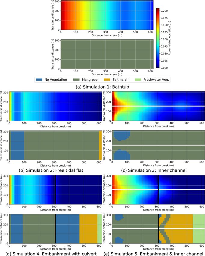
772                     A. Breda et al.: Accretion, retreat and transgression of coastal wetlands experiencing sea-level rise

Figure 1. Field site and areas within the site characterised by the numerical simulations: (a) Area E of Kooragang wetlands, (b) areas within
the wetland where the simplified simulations represent the dominant processes, (c) schematic longitudinal view of the domain setup and
sinusoidal wave input (adapted from Rodriguez et al., 2017), and (d) schematic isometric view of each simulated domain and their hydraulic
features. Vegetation cover is only indicative and roughly corresponds to early stages of the simulations. Elevation unit, mAMSL, stands for
metres above mean sea level.

computed as an average of the values at cells k and i, and               is 0.12 s m−1/3 , while for the channel cell it is 0.035 s m−1/3 .
xk − xi is the distance between cells. Based on Rodriguez                For cells in the channel, the full momentum equation is
et al. (2017) we adopt roughness coefficients for mangrove               used to account for dynamic and backwater effects (Riccardi,
and saltmarsh cells of 0.50 s m−1/3 and 0.15 s m−1/3 respec-             2000). If the domain includes a culvert at cell i, then the dis-
tively. For freshwater and non-vegetated cells, Manning’s n

Hydrol. Earth Syst. Sci., 25, 769–786, 2021                                                 https://doi.org/10.5194/hess-25-769-2021

A. Breda et al.: Accretion, retreat and transgression of coastal wetlands experiencing sea-level rise                            773

charge between cells k and i is computed as                        erage sediment concentration in the water column and the
             1          1                                          water depth. Here, we use a more physically based equa-
       (2g) (zk − zi )
             2          2
                                                                   tion for fine sediment transport and deposition processes cou-
Qk,i =            1 ,                                     (3)
                       2                                           pled to the hydrodynamic simulations. The sediment model
           1     1
          2 2 − 2
          Cd Ai    Ak                                              solves the quasi-two-dimensional continuity equation of sus-
                                                                   pended sediment neglecting horizontal diffusion (Garcia et
in which Ai and Ak are respectively the cross-sectional ar-        al., 2015). The continuity equation for the ith cell reads as
eas at the i and k cells and Cd is a standard discharge co-        follows:
efficient for the culvert at cell i adopted as 0.8. Equation (3)
                                                                        d(hC)i              Xj
considered the case of the culvert flowing under the influence     Asi           = Asi ϕi +        (QC)k,i ,                  (4)
                                                                          dt                   k=1
of gravity. For pressurised conditions, a different equation is
used (Riccardi, 2000).                                             where hi is the water depth of cell i (m); Ci is the sediment
   The model equations are solved using an implicit method         concentration (g m−3 ), ϕi is the downward vertical flux of
and a Newton–Raphson algorithm. The time step used in the          fine sediment (g m−2 s−1 ), and Ck,i are the sediment concen-
model solution is 1 s to ensure numerical stability. Further       trations in the j neighbouring cells. For fine-grained sedi-
explanation about the application of this model in a similar       ment typical of estuarine environments, the downward flux
EGM framework can be found in Sandi et al. (2018).                 can be expressed as (Krone, 1962; Mehta and McAnally,
                                                                   2008)
2.3   Vegetation model
                                                                                    τbi
                                                                   ϕi = −ws 1 −           C i ; τb < τ d ,                   (5)
Vegetation in coastal wetlands is driven by the tidal regime,                        τd
so we use water depth time series to compute the mean depth
below high tide, D, and the hydroperiod, H , on every cell         where ws is the fall/settling velocity of suspended sediment
as a descriptor of the tidal regime. These variables are the       particles (m s−1 ), τbi is the magnitude of bed shear stress in
input for all the other models of the EGM framework. The           cell i (Pa), and τd is the critical bed shear stress for deposition
first variable represents the average maximum water depth on       (Pa). Velocities were converted to bed shear stresses using
spring tides. In this case we use a sinusoidal wave, so D is the   τbi = ρ Cf Ui2 .                                               (6)
maximum depth. The hydroperiod accounts for the duration
of the inundation period and is computed as the proportion of      In Eq. (6) ρ is the water density and Cf is a friction coeffi-
time during which a minimum water depth is present during          cient set at 0.05. The parameters ws and τd were varied to re-
the simulation time.                                               produce similar levels of accretion observed in the wetlands
   The values of H and D define the suitable conditions for        where the original modelling framework was applied (Ro-
vegetation establishment and survival at each point in the         driguez et al., 2017). The values obtained were τd = 0.02 Pa
wetland based on thresholds that have been tested for south-       and ws = 2×10⁻⁴ m s−1 , which are consistent with values re-
eastern Australian estuaries (Rodriguez et al., 2017). Thus,       ported by Larsen et al. (2009) and Temmerman et al. (2005).
the observed threshold applies to Avicennia marina (grey           This model does not have an erosion term, which is not a bad
mangrove) and to a composition of saltmarsh species Sar-           simplification over vegetated surfaces that receive flows that
cocornia quinqueflora and Sporobolus virginicus. Mangrove          are typically very slow.
depends primarily on hydroperiod, requires frequent inunda-           Equation (4) is solved using the same numerical scheme
tions and establishes itself in areas where 10 % < H < 50 %        than the water mass conservation (Eq. 1), providing a time
and D > 0.2 m, where H is calculated as the fraction of            series of sediment concentrations in each cell of the domain.
time where the water depth is higher than or equal to 14 cm,       However, as the soil elevation model (next section) works at
the typical height of the pneumatophores. Saltmarsh toler-         a larger timescale and requires the annual concentration, C̄,
ates prolonged inundations and can survive in areas where          a weighted average is computed for each cell:
H < 80 % but cannot endure inundation depths above its                   PM
height (25 cm), so we limit D < 0.25 m. We consider that, if                    (Ct × ht )
                                                                   C̄ = t=0  PM            ,                                  (7)
conditions suit both mangrove and saltmarsh, mangrove will                      t=0 ht
expand over saltmarsh areas (Saintilan et al., 2014). In areas
not exposed to saltwater (H = 0 %, D ∼ 0 m), we assume the         where t is the time in the hydrodynamic simulation with M
presence of freshwater vegetation, and if none of the above        the final step; Ct and ht are the sediment concentration and
conditions applies, areas are considered to be non-vegetated.      the water depth respectively at time t.
                                                                      The sediment transport equation based on mass conserva-
2.4   Sediment model                                               tion (Eq. 4) cannot be used in the case of the bathtub simu-
                                                                   lations because the bathtub model does not provide informa-
The original version of the framework used in the Hunter           tion on water discharge and velocity. For the bathtub sim-
estuary applies a linear empirical relationship between av-        ulations, we used the linear relation between water depth

https://doi.org/10.5194/hess-25-769-2021                                              Hydrol. Earth Syst. Sci., 25, 769–786, 2021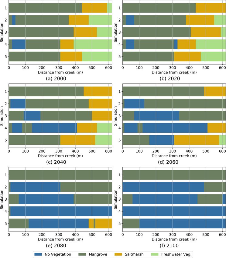
774                   A. Breda et al.: Accretion, retreat and transgression of coastal wetlands experiencing sea-level rise

and concentration empirically developed by Rodriguez et          Table 1. Parameters of the soil surface elevation model.
al. (2017). Based on the measured data, the fitted equation
is                                                                          Model parameter      Mangrove       Saltmarsh
                                                                            a (g m−4 )            −6037.6        −16 767
C̄ = Cmax (0.55D + 0.32),                                  (8)
                                                                            b (g m−3 )              7848.9          8384
where C̄ is the average sediment concentration (g m−3 ), and                c (g m−2 )            −1328.3              0
Cmax is the concentration at the wetland inlet.                             q (m3 yr−1 g−1 )      9 × 10⁻⁵      9 × 10⁻⁵
   This equation is much simpler and has different parame-                  k (m5 g−2 )         1.2 × 10⁻⁷    6.2 × 10⁻⁷
ters than the sediment transport equation; however, for very
simple flow conditions it should produce comparable results.
We confirmed the suitability of the simple model by compar-      is noisy and varies considerably over very short distances. In
ing EGM results using the bathtub approach (with the lin-        order to work with a more realistic distribution of deposition
ear sediment relation) and a full hydrodynamic and sediment      over the tidal flat, we smooth the topography by applying a
transport EGM over a smooth topography. Both the hydro-          very simple diffusion model. The diffusion model does not
dynamics and the resulting elevation changes of both models      change the general trends of deposition and avoids localised
were very similar (see Fig. S1 in the Supplement).               peaks of excessive deposition.

2.5   Soil elevation change model
                                                                 3     Results
Our EGM framework adopts the model originally proposed
by Morris et al. (2002) and later modified by Kirwan and         3.1    Spatial patterns of accretion and vegetation
Guntenspergen (2010) to estimate the increase in soil eleva-
tion due to accretion as a function of hydrodynamic and eco-     In order to show the characteristic spatial patterns of each of
logical conditions. We first compute the biomass production,     the typical cases analysed, we first show in Fig. 2 accumu-
B (g m−2 ), by using the parabolic equation                      lated accretion (1E) and vegetation distribution in 2050 un-
                                                                 der the expected SLR scenario for each of the five numerical
B = aD 2 + bD + c,                                         (9)   simulations, including the bathtub and the other four simula-
                                                                 tions that use a hydrodynamic and sediment transport (HST)
where a, b, and c are parameters fitted to field data, for       model. Details on the temporal evolution of topography and
each vegetation type. Then, the surface elevation change rate,   vegetation for each of the simulations are provided later in
dE/dt (m yr−1 ), is calculated using                             the paper.
dE                                                                  Figure 2 shows that accumulated accretion is homoge-
   = C̄ (q + kB) D,                                      (10)    neous in the transverse direction for the simulations without
dt
                                                                 the channel (Fig. 2a, b, d), as there is no lateral flow and the
where q is a depositional parameter and k is a vegeta-           changes in sedimentation occur in the longitudinal direction
tion sediment trapping coefficient. For all five parameters of   only. For the simulations with the central drainage channel
Eqs. (9) and (10) we used the values adopted in Rodriguez et     (Fig. 2c, e) there is a marked concentration of flow and sed-
al. (2017) and Sandi et al. (2018) (see Table 1) for an Aus-     iment accumulation close to the channel. Some of the accu-
tralian wetland. Although the term Asi ϕi in Eq. (4) provides    mulated accretion patterns of the simulations with the chan-
an amount of settled sediment that contributes to accretion,     nel presented in Fig. 2 are remarkably similar to the results
it only considers the gravitational settling of sediment and     from Chen et al. (2010) on a similar geometry.
does not include many other important accretion processes           It can be seen from the figure that all simulations show
associated with the presence of vegetation. The full effects     a general decrease in accretion with distance to the tidal in-
of sediment and vegetation are considered in Eq. (10), which     put (which can represent a tidal creek or the river), which is
produces much larger accretion values (see Fig. S2 in the        expected because the source of sediment is at the tidal in-
Supplement).                                                     put. However, each simulation has a characteristic elevation
   The EGM simulations use a yearly time step; i.e. the com-     profile and vegetation distribution, and they are all quite dif-
puted biomass and accretion represent an average condition       ferent from the predictions of the bathtub model. Figure 2a
within this period. We choose a yearly time step as vegeta-      shows that the bathtub simulation displays a smoother and
tion dynamics does not respond instantaneously to flow and       longer transition of accumulated accretion. A slight concen-
depositional processes (Alizad et al., 2016b; Saco and Ro-       tration of accretion is observed at 500 m from the creek due
dríguez, 2013; Schuerch et al., 2018). Our model does not        to the initial position of high biomass saltmarsh. The bathtub
account for erosion and diffusion processes and also does not    case has flood and ebb flows of the same duration, since there
take into account the redistribution of deposited sediment by    is no flow attenuation. This keeps the hydroperiod within a
waves. Because of that, the resulting accretion from Eq. (10)    range that promotes mangrove establishment over most of the

Hydrol. Earth Syst. Sci., 25, 769–786, 2021                                         https://doi.org/10.5194/hess-25-769-2021
A. Breda et al.: Accretion, retreat and transgression of coastal wetlands experiencing sea-level rise                              775

Figure 2. Accumulated accretion (top) and vegetation maps (bottom) in 2050 for low sediment input corresponding to (a) Simulation 1, (b)
Simulation 2, (c) Simulation 3, (d) Simulation 4, and (e) Simulation 5.

wetland. Saltmarsh is limited to the upper parts of the tidal         to the tidal input than the bathtub simulation. In Simulation 3
flat.                                                                 (Fig. 2c), the inner channel increases the drainage of the sur-
   The other simulations (2 to 5) use the hydrodynamic and            rounding areas, thus reducing the hydroperiod in the vicinity
sediment transport (HST) models instead of the bathtub ap-            of the channel and allowing mangroves to persist close to
proximation. In these cases, accretion presents an exponen-           the tidal creek. The channel also enhances sediment delivery
tial shape with a sharper decrease than the bathtub model,            farther from the tidal input, which causes an increase in ac-
and vegetation establishment is strongly controlled by the ef-        cretion around the mid-point of the flat (300 m from the tidal
fects of vegetation roughness, channel and culverts. In con-          creek). However, this effect is concentrated near the chan-
trast to the bathtub model results, all HST simulations show          nel and fades away as flow is directed into the tidal flat. In
mangrove dieback in lower areas, which is caused by a higher          Simulation 4 (Fig. 2d), the flow is restricted by an embank-
hydroperiod due to attenuated ebb flows.                              ment and a culvert, so the hydroperiods in the upper wetland
   Simulation 2, with the undisturbed tidal flat (Fig. 2b),           are higher. This effect reduces mangrove migration and its
shows the effect of hydraulic resistance due to the vegetation        encroachment on saltmarsh areas. In Simulation 5 with em-
roughness only, which generates an elevation mound closer             bankment and channel (Fig. 2e), the channel promotes man-

https://doi.org/10.5194/hess-25-769-2021                                               Hydrol. Earth Syst. Sci., 25, 769–786, 2021
776                   A. Breda et al.: Accretion, retreat and transgression of coastal wetlands experiencing sea-level rise

grove landwards of the embankment and also the stabilisa-         but with larger values of accumulated accretion were ob-
tion of saltmarsh areas in the upper sections of the tidal flat   tained for a higher sediment input of 111 g m−3 (Fig. S3 in
as they receive more sediment (Fig. 2e).                          the Supplement).
                                                                     The reduction in accretion in the simulations that consider
3.2   Evolution of accumulated accretion profiles                 the actual features of the wetland can be better appreciated in
                                                                  Fig. 4, in which we compare domain-average 1E of all sim-
Figure 3 shows the results of surface elevation change (1E)       ulations over time. Fig. 4 includes results for a low sediment
in each simulation for the years 2020, 2040, 2060 and 2100        input of 37 g m−3 (Fig. 4a) and for a high sediment input of
for low sediment input conditions (corresponding to contem-       111 g m−3 (Fig. 4b). The figure also includes the values of
porary rates in the Hunter estuary), in terms of accumulated      mean sea level for each year to give an idea of the submer-
accretion profiles along the main flow direction. For the sim-    gence conditions in the wetlands.
ulations with the central drainage channel (Simulations 3 and        There is a clear difference between the accretion gener-
5), we have included two profiles at different transverse lo-     ated in the bathtub simulation and the rest of the simulations.
cations, one close to the channel and one 150 m away in the       In our simulations, accretion is a function of sediment con-
middle of the tidal flat.                                         centration and depth below mean high tide (D). The bathtub
   During the first 2 decades, the vegetation type plays an       assumption overpredicts both inputs over the entire domain,
important role in the longitudinal distribution of the accu-      thus generating higher accretion values. In all HST simula-
mulated accretion profiles. By 2020 (first column of Fig. 3)      tions, the combination of a reduction in D because of flow
the profiles show a continuous decrease from the tidal input      attenuation and the exponential decay of sediment concen-
up to 300 to 350 m approximately, which coincides with the        tration results in less accretion than in the bathtub simula-
transition from mangrove to saltmarsh in the initial vegeta-      tion. In the case of low sediment input (Fig. 4a), by 2050 the
tion distributions (see Fig. 5 later in the paper). This occurs   domain-average 1E from the bathtub is about 2 times the
due to the dynamics of sediment transport (more deposition        values of all the other simulations, increasing to more than 3
close to the tidal input) and also due to the reduction of the    times by 2100. In the simulations with high sediment input
mangrove biomass away from the tidal creek (reductions in         (Fig. 4b), the accumulated accretions of bathtub simulations
D; see Eq. 10). The increase in 1E at the transition is due       are 2.5 and 4 times the values of the rest of the simulations
to the saltmarsh having a higher biomass and trapping effi-       for 2050 and 2100 respectively. The simulations with the
ciency than mangrove at that particular value of D. Landward      HST simulations present different levels of attenuation and
of the transition, 1E decreases with decreases in saltmarsh       accordingly different accretion levels. The lowest accretion
biomass. This general dynamics is disrupted by the presence       corresponds to the highly attenuated case with embankment
of the culvert because it limits the amount of sediment reach-    and culvert (Simulation 4), whereas the highest accretion oc-
ing the upper areas of the tidal flat.                            curs in the case of the central channel (Simulation 3) that ex-
   Changes in 1E slow down after 2060 in all simulations          periences increased drainage and thus less attenuation. The
except for the bathtub case. This is due to reductions in veg-    cases of the tidal flat with no structures (Simulation 2) and of
etation as most of the lower areas of the tidal flat have expe-   the embankment with the inner channel (Simulation 5) have
rienced submergence and vegetation loss. Small increases in       intermediate levels of attenuation and accretion.
1E occur in the upper areas in the cases in which the central        All simulations show a strong elevation deficit (i.e. the dif-
channel promotes tidal flushing (Simulations 3 and 5), but        ference between the rate of sea-level rise and wetland ac-
this effect is concentrated in areas close to the channel.        cretion rate dE/dt), as none of the simulations predict that
   None of the simulations using the HST model produces           the tidal flat is capable of keeping pace with SLR. For the
1E results similar to the bathtub simulations. The simula-        low-sediment conditions, by 2050 the elevation deficit of the
tion with the central channel (Simulation 3) presents values      bathtub simulation is 5.5 mm yr−1 , while the rest of the sim-
of 1E near the channel that are close to the results of the       ulations predict an elevation deficit of about 7 mm yr−1 . Over
bathtub simulation during the first years, but over time, the     time, the elevation deficits increase and by 2100 the bathtub
results diverge. The increased 1E values are limited to areas     predictions reach a value of 9.5 mm yr−1 and the HST simu-
next to the channel, and they quickly decline as the flow is      lations a value of 12 mm yr−1 .
directed into the tidal flat. In general, the outcomes from the      Increasing the sediment input concentration considerably
HST model show a reduction in the water levels and total ac-      changes the accretion capacity of the tidal flat, particularly
cretion compared to the bathtub results. Furthermore, when        according to the bathtub results. Bathtub simulations pre-
the culvert is introduced in the simulation (Simulations 4 and    dict that the tidal flat is able to accrete at a rate that al-
5), the main effect is a drastic reduction of 1E in the upper     most matches the changes in sea level, so the wetland sur-
areas of the domain.                                              vives sea-level rise. Accretions for all other simulations are
   Figure 3 results correspond to a situation with a low sedi-    moderate, with the simulations that have the central chan-
ment input of 37 g m−3 , typical of current south-eastern Aus-    nel (Simulations 3 and 5) responding more effectively to the
tralian conditions (Rodriguez et al., 2017). Similar patterns     increased sediment and accreting more than the other simu-

Hydrol. Earth Syst. Sci., 25, 769–786, 2021                                         https://doi.org/10.5194/hess-25-769-2021
A. Breda et al.: Accretion, retreat and transgression of coastal wetlands experiencing sea-level rise 777 Figure 3. Longitudinal profiles of accumulated accretion (1E, m) for a sediment supply of 37 g m−3 . The vertical black line represents the embankment with culvert. The “channel” profile represents the elevation gain near the central channel, while the “tidal flat” profile is situated in the middle of the tidal flat. Note: simulation starts in the year 2000. lations (Simulations 2 and 4). Compared to the low sediment a drainage channel together with the embankment and culvert conditions, elevation deficits of the bathtub predictions re- (Simulation 5) represents an intermediate situation in which duce to 3 and 5.5 mm yr−1 by 2050 and 2100 respectively, the increased flushing effect of the channel and the attenuat- while in the other simulations those values increase to about ing effect of the embankment and culvert partially compen- 6 and 10 mm yr−1 . sate. The structures included in the simulations have a clear ef- In Fig. 4a we have also included the average accumulated fect on the average 1E. The inner channel promotes accre- accretion for the entire wetland site (Area E in Fig. 1b) us- tion further inland, as it conveys more water and sediment ing information from Rodriguez et al. (2017) and Sandi et to those areas away from the tidal input. Compared to the al. (2018). Rodriguez et al. (2017) applied a similar EGM tidal flat free of structures (Simulation 2), the inclusion of formulation to Area E (Fig. 1c) to assess the effect of at- the channel (Simulation 3) is responsible for an increase in tenuation on wetland evolution under SLR considering typ- wetland-accumulated accretion of about 50 %. The opposite ical (37 g m−3 ) and increased (111 g m−3 ) sediment condi- effect is observed when the embankment with culvert is in- tions. Sandi et al. (2018) further studied the effects of tidal troduced, as it attenuates and reduces the water and sediment restrictions at the wetland inlet considering typical sediment flow into the upper part of the wetland. Comparing results loads. The values included in the figure correspond to aver- for the tidal flat without (Simulation 2) and with (Simulation age accumulated accretion over the entire wetland at 2050 4) embankment and culvert, we can observe a reduction in and 2100 for low sediment load with and without tidal re- wetland-accumulated accretion of 25 %. The introduction of strictions (Fig. 4a) and for high sediment load without restric- https://doi.org/10.5194/hess-25-769-2021 Hydrol. Earth Syst. Sci., 25, 769–786, 2021
778                    A. Breda et al.: Accretion, retreat and transgression of coastal wetlands experiencing sea-level rise

Figure 4. Sea-level rise and domain-average accumulated accretion over time for all simulations for (a) low sediment input and (b) high
sediment input. Results from Rodriguez et al. (2017) and Sandi et al. (2018) corresponding to the entire Area E wetland are included for
comparison.

tions (Fig. 4b). The figures show that the simulations without        dation in the upper areas, reducing the extent of the saltmarsh
tidal restrictions result in values of accumulated accretion          to about 100 m from the embankment.
similar to the simulation with low attenuation (Simulations              After 20 years (Fig. 5b) Simulations 1, 2 and 3 show man-
3 and 5) for both low and high sediment loads, while predic-          grove encroachment on saltmarsh. The upstream mangrove
tions of accumulated accretion including tidal restrictions are       edge moves up to 50 m, forcing saltmarsh occurrence in ar-
closer to the simulation with high attenuation (Simulations 2         eas further than 300 m from the tide input creek. In Simula-
and 4).                                                               tions 4 and 5 the embankment halts mangrove migration and
                                                                      increases in inundation of upper areas promote saltmarsh in-
3.3   Changes in vegetation                                           crease. Overall, wetland area increases due to mangrove ex-
                                                                      pansion (Simulations 1, 2 and 3) or to saltmarsh expansion
The interactions between sea-level rise, accretion and vege-          (Simulations 4 and 5).
tation changes are complex because vegetation not only re-               By 2040 (Fig. 5c), mangrove has encroached further on
sponds to vertical elevation changes, but also migrates in-           saltmarsh in Simulations 1, 2 and 3, resulting in saltmarsh
land. In order to obtain a clear picture of the vegetation            squeeze at the upper end due to the landward boundary of the
changes over time, we simplified two-dimensional vegeta-              computational domain. Simulations 4 and 5 show very minor
tion maps (i.e. Fig. 2) into a one-dimensional representation.        encroachment of mangrove on saltmarsh, which is able to
The vegetation type at a given distance from the tidal input          migrate landward. Total wetland area remains approximately
was determined by selecting the predominant (higher occur-            unchanged for Simulations 1, 2 and 3, while it keeps increas-
rence) vegetation in the transverse direction. Figure 5 shows         ing in Simulations 4 and 5. Some areas of mudflat start ap-
snapshots of the predominant vegetation every 20 years. As            pearing in the HST simulations due to extended hydroperi-
already explained, in the simulations with embankment and             ods.
culvert (Simulations 4 and 5), the structures are located at             Twenty years later, in 2060 (Fig. 5d), the MSL is about
310 m from the tidal input. The conditions at the beginning           30 cm higher than in 2000, and we can see considerable mud-
of the simulation (Fig. 5a) for Simulations 1, 2 and 3 show           flat areas in all simulations except for the bathtub simulation
mangrove occupying approximately the lower 400 m of the               (Simulation 1), which presents a uniform coverage of man-
tidal flat and saltmarsh the next 200 m upland. For Simula-           grove over the entire domain. Saltmarsh is totally absent in
tions 4 and 5 the presence of the embankment reduces hy-              Simulations 1, 2 and 3 due to mangrove encroachment but
droperiods in the upper areas, constraining mangrove to the           still remains almost unchanged in Simulations 4 and 5. All
lower 310 m. The embankment also limits the extent of inun-           simulations except the bathtub simulation show decreases

Hydrol. Earth Syst. Sci., 25, 769–786, 2021                                              https://doi.org/10.5194/hess-25-769-2021
A. Breda et al.: Accretion, retreat and transgression of coastal wetlands experiencing sea-level rise 779 Figure 5. Predominant position occupied by each vegetation type in the tidal flat from 2000 to 2100. Simulations for low sediment input, SSC = 37 g m−3 . Simulations: 1 Bathtub, 2 Free tidal flat, 3 Inner channel, 4 Embankment with culvert and 5 Embankment and inner channel. in wetland extent, mostly due to saltmarsh disappearance in losses in their simulations with tidal input restrictions at the Simulations 2 and 3 and to mangrove squeeze in Simulations wetland inlet when compared to the case without restrictions. 4 and 5. The same analysis of vegetation evolution for the high sed- From 2080 on (Fig. 5e, f), a rapid retreat of the remain- iment input scenario is presented in Fig. 6. With increased ing wetland can be observed in all simulations. The retreat sediment, the patterns of vegetation change remain remark- occurs faster for the simulations with the embankment, re- ably similar to the patterns observed in Fig. 5 for the low sulting in total wetland disappearance by 2100. The rest of sediment conditions, with the exception of the bathtub sim- the simulations still show some remnant mangrove areas by ulations (Simulation 1). Compared to Fig. 5, the bathtub re- 2100, which are only significant (40 %) in the case of the sults indicate that saltmarsh is able to remain in the upper bathtub simulations. wetland areas for longer (until 2060) and that mangrove does The same trend of increase in wetland area in the first 20 not retreat, resulting in no wetland loss after 100 years of years of simulation, followed by a continuous decrease start- simulation. The other simulations without embankment (2 ing at 40 years and ending at 100 years with almost complete and 3) show a slightly slower retreat of both mangrove and wetland disappearance under the same sea-level rise trajec- saltmarsh than in Fig. 5, while the simulations with the em- tory, was observed by Rodriguez et al. (2017) and Sandi et bankment show almost the same behaviour as in the case of al. (2018). Sandi et al. (2018) also reported larger wetland low sediment. Some of the simulations in Fig. 6 show lo- https://doi.org/10.5194/hess-25-769-2021 Hydrol. Earth Syst. Sci., 25, 769–786, 2021
780                    A. Breda et al.: Accretion, retreat and transgression of coastal wetlands experiencing sea-level rise

calised mangrove areas that tend to establish themselves and        due to low accretion rates has been reported before (Kirwan
persist close to the tidal creek.                                   et al., 2010; Lovelock et al., 2015b; Rodriguez et al., 2017;
   For a more detailed analysis, we can look at the vegetation      Sandi et al., 2018; Schuerch et al., 2018). However, the re-
evolution in terms of wetland area (mangrove and saltmarsh),        sults for high sediment load seem to challenge some previous
wetland retreat (position of the seaward edge) and wetland          studies highlighting the potential of biophysical feedbacks to
transgression (position of the landward edge).                      produce accretion rates comparable to SLR (D’Alpaos et al.,
   Figure 7a shows that the wetland extent predicted using          2007; Kirwan and Murray, 2007; Kirwan et al., 2016b; Mudd
the bathtub approach (Simulation 1) is affected by the sedi-        et al., 2009; Temmerman et al., 2003). In our case, the bio-
ment load, with only the low sediment condition resulting in        physical feedbacks with a high sediment load produced wet-
a sharp decay in extent after 2060/70. The difference in ex-        land accretion rates similar to SLR rates only for the bathtub
tent is due to the vegetation retreat in the low sediment case,     simulation.
which does not occur in the high sediment case (Fig. 7b).              Analysis of accretion rates indicates that all simulations
Wetland extent values for the HST simulations are not greatly       start with similar rates in the vegetated areas, with about
affected by the sediment load, and they are much smaller than       2.5 and 7.5 mm yr−1 in the low and high sediment situa-
the values predicted by the bathtub (Fig. 7a). Wetland retreat      tions respectively. For the low sediment case, the initial value
starts first in the simulations without the channel (Simula-        compared very well with historic values for south-eastern
tions 2 and 4) and about 20 years later in the simulations with     Australian conditions measured by Howe et al. (2009) and
the channel (Simulations 3 and 5) due to increased drainage.        Rogers et al. (2006). For the high sediment case, an increase
Once the retreat starts, it occurs faster in the simulations with   in the accretion value by a factor of 3 seems reasonable con-
the embankment (Simulations 4 and 5) that delays the ebb            sidering an increase in the sediment load by a factor of 3
flows and increases hydroperiods in the lower wetland areas.        (from 37 to 111 g m−3 ). Those starting values of accretion
   Wetland transgression is not affected by the sediment con-       remain at approximately the same level over most of the time
ditions (Fig. 7c) because of the limited amount of sediment         for the bathtub simulations, while they decrease for the HST
that reaches the upper wetland areas. Transgression starts          simulations. The decrease is more marked for Simulations
later in the simulations with the embankment (Simulations           2 and 4 (which reach a value of about 1 to 1.5 mm yr−1 by
4 and 5) because of the reduced depths and sediment loads in        2050) than for the simulations with inner channel Simula-
the upper wetland areas. The presence of the channel (Simu-         tions 3 and 5 (which attain values of 2 and 4 mm yr−1 by
lations 3 and 5) results in earlier but more gradual transgres-     2050 for low and high sediment conditions respectively). The
sion compared to setups with no drainage structure (Simula-         reduction of the magnitude of the biophysical feedbacks over
tions 2 and 4).                                                     time is due to the continuous upland migration of vegetation,
                                                                    which colonises upper areas with comparatively less water
                                                                    depth and sediment supply (see also Sandi et al., 2018). The
4   Discussion                                                      bathtub model predicts less migration and higher depths, so
                                                                    it consistently overestimates accretion rates.
The interactions between all the processes related to the dy-          Despite having reduced accretion rates when compared to
namics of coastal wetlands are quite complex (Fagherazzi et         the bathtub simulations, the HST simulations still show a no-
al., 2012; Reef et al., 2018; Saintilan et al., 2014), which        ticeable difference in elevation gains depending on the sedi-
makes the bathtub assumption limited for most applications.         ment supply levels. Compared to the low sediment case, the
Places with multiple vegetation species (Cahoon et al., 2011;       high sediment supply case results in about twice the average
Rogers et al., 2006) and an intertwined channel network             accumulated accretion (Fig. 4). However, analysis of vege-
(D’Alpaos, 2011) present a strong heterogeneity of saltwa-          tation changes over time for low (Fig. 5) and high (Fig. 6)
ter exposure and sediment delivery to the overbank areas            sediment loads reveals minimum differences between them.
that need a detailed description of flow and sediment pro-          Analysis of Fig. 7 shows that even though the increase in
cesses (see also Coleman et al., 2020). Artificial structures       sediment load generates about twice the accretion, this extra
constraining flow and sediment modify accretion rates (Bel-         elevation is not sufficient to prevent wetland submergence.
lafiore et al., 2014; Cahoon et al., 2011) and thus wetland         Figure 4 suggests that accretion rates of 4 times the historic
evolution (Rodriguez et al., 2017; Sandi et al., 2018). Even        values or more are needed for the wetlands to be able to cope
though our simulation design focused on simplified setups,          with SLR.
these setups comprise typical wetland features and include             Although the simulations carried out in this study were
most of the complex processes and interactions.                     conducted on simplified domains, they can capture the gen-
   Our results indicate that wetlands do not cope with              eral response of more complex domains present in real wet-
SLR for the simulated conditions corresponding to a high-           lands, as shown by the comparison with entire wetland re-
emission climate change scenario. This result was not sur-          sults from Rodriguez et al. (2017) and Sandi et al. (2018) in
prising for the low sediment situation, as the inability of         Fig. 4. Moreover, the features included are present in many
sediment-poor coastal wetlands to survive high levels of SLR        coastal areas around the world and thus have wider implica-

Hydrol. Earth Syst. Sci., 25, 769–786, 2021                                           https://doi.org/10.5194/hess-25-769-2021
A. Breda et al.: Accretion, retreat and transgression of coastal wetlands experiencing sea-level rise 781 Figure 6. Predominant position occupied by each vegetation type in the tidal flat from 2000 to 2100. Simulations for high sediment input, SSC = 111 g m−3 . Simulations: 1 Bathtub, 2 Free tidal flat, 3 Inner channel, 4 Embankment with culvert and 5 Embankment and inner channel. tions. Our bathtub results for low sediment conditions pre- et al., 2015; Kirwan and Megonigal, 2013), so we can ex- dicting an initial increase in wetland extent early in the cen- pect a behaviour closer to that of Simulations 4 and 5. On the tury and then a decrease after 2060 agree with previous bath- other hand, wetlands with dense drainage networks like the tub model predictions (Lovelock et al., 2015b; Rogers et al., Venice Lagoon in Italy (Silvestri et al., 2005), the Scheldt 2012; Schuerch et al., 2018). However, using the HST frame- estuary in the Netherlands (Temmerman et al., 2012), and work, our predictions indicate that the decrease may start as the North Inlet in South Carolina, US (Morris et al., 2005), early as 2030 for wetlands with a tidal range close to 1.3 m would probably behave similarly to Simulation 3 and experi- (as represented in our study), over a wide range of sediment ence comparatively smaller losses of area. loads. We can expect that this accelerated wetland loss will The results presented in this study show generalised con- affect many parts of the world, particularly in areas with mi- ditions of wetland dynamics under sea-level rise by using cro to meso tidal ranges and heavily developed coasts, like several simplified domains that focus on individual mecha- eastern Australia (Williams and Watford, 1997), parts of the nisms affecting ecogeomorphic evolution. This approach can eastern US (Crain et al., 2009), the western US (Thorne et al., support a broader perspective of the potential fate of coastal 2018), eastern China (Tian et al., 2016) and western Europe wetlands in general, but some limitations arise as part of the (Gibson et al., 2007). In these environments, attenuation can model assumptions. As with most wetland evolution models, be important due to manmade structures, and transgression we did not consider soil processes other than accretion, dis- may be limited by development (Doody, 2013; Geselbracht regarding swelling, compaction and deep subsidence. Mea- https://doi.org/10.5194/hess-25-769-2021 Hydrol. Earth Syst. Sci., 25, 769–786, 2021
782                   A. Breda et al.: Accretion, retreat and transgression of coastal wetlands experiencing sea-level rise

Figure 7. Time evolution of wetland in low (SSC = 37 g m−3 ) and high (SSC = 111 g m−3 ) sediment environments under SLR. (a) Wetland
area; (b); wetland retreat; and (c) wetland transgression.

surements in wetlands of the Hunter estuary show that long-          velocities. We believe that in our case excluding storm effects
term surface elevation changes are mostly due to accretion,          is justifiable based on Rogers et al. (2013), who found that in
supporting our assumption (Howe et al., 2009; Rogers et al.,         these fine sediment environments storms affect accretion dy-
2006). Another process that we did not consider was the              namics over the short term (immediate erosion or low accre-
effects of marsh edge retreat due to ocean or wind waves             tion followed by increased deposition over the next months),
(Carniello et al., 2012; Fagherazzi et al., 2012), which can         but they do not change the long-term trend of accretion and
have a significant role in coastal wetland evolution. Most           elevation gain rates.
coastal wetlands in Australia are estuarine and not exposed to
ocean waves, whereas wind effects in our wetland were not
important due to the absence of large open water areas where         5   Conclusions
wind waves could fully develop. We also simplified the tidal
signal without including neap–spring cycles, which sped up           We conducted detailed numerical simulations on the re-
computations but which may have affected the results. How-           sponse to SLR of four different typical coastal wetland set-
ever, preliminary tests including neap–spring tide variability       tings, including the case of a vegetated tidal flat free from ob-
showed only small differences in the initial landward edge of        structions and drainage features and three other settings that
saltmarsh, which did not affect the accretion dynamics due           included an inner channel, an embankment with a culvert,
to the small depths and low sediment availability in that area.      and a combination of inner channel, embankment and cul-
Finally, our simulations did not include the effect of storms,       vert. We also included a simulation using a simple bathtub
which can influence sediment availability, water depths and          approach, in which none of the features (vegetation, chan-

Hydrol. Earth Syst. Sci., 25, 769–786, 2021                                            https://doi.org/10.5194/hess-25-769-2021
A. Breda et al.: Accretion, retreat and transgression of coastal wetlands experiencing sea-level rise                                   783

nels, culverts) are considered. We used conditions typical of         PMS, SGS, GR and NS analysed the results. AB, PMS and JFR
south-eastern Australia in terms of vegetation, tidal range and       wrote the paper with substantial input from all the co-authors.
sediment load, but we also analysed simulations with an in-
creased sediment load to assess the potential of biophysical
feedbacks to enhance accretion rates.                                 Competing interests. The authors declare that they have no conflict
   We found that the distinct patterns of flow and sediment           of interest.
redistribution obtained from these simulations result in in-
creased wetland vulnerability to SLR when compared to pre-
dictions using the simple bathtub approach. Changes in el-            Acknowledgements. Patricia M. Saco is grateful for support from
                                                                      the Australian Research Council (grant no. FT140100610). An-
evation due to accretion were between 10 % and 50 % of
                                                                      gelo Breda was supported by a University of Newcastle PhD schol-
those obtained from bathtub predictions, and wetland retreat          arship.
and reduction of wetland extent started 20 to 40 years earlier
than for the case of the bathtub simulations, depending on
wetland setting. Transgression for all settings was delayed           Financial support. This research has been supported by the Aus-
with respect to the bathtub predictions and was limited by            tralian Research Council (grant no. FT140100610) and the Univer-
the presence of a hard barrier at the upland end.                     sity of Newcastle Australia (PhD scholarship).
   The simulations using the full hydrodynamic and sediment
transport dynamic models indicated that wetlands with good
drainage (e.g. including an inner channel) were more resilient        Review statement. This paper was edited by Nadia Ursino and re-
to SLR, displaying more accretion, a later retreat and reduc-         viewed by two anonymous referees.
tion of wetland area and an increased transgression when
compared with wetlands with strong flow impediments (e.g.
including an embankment).
   Increasing the sediment load delivered to the wetlands by          References
a factor of 3 increased the accretion of all wetland settings by
a factor of 2. However, this extra elevation was not enough           Alizad, K., Hagen, S. C., Morris, J. T., Bacopoulos, P., Bil-
                                                                         skie, M. V., Weishampel, J. F., and Medeiros, S. C.: A
to prevent wetland submergence, as predictions of wetland
                                                                         coupled,      two-dimensional        hydrodynamic-marsh        model
evolution were very similar for low and high sediment condi-
                                                                         with biological feedback, Ecol. Model., 327, 29–43,
tions. Based on our results, we estimate that accretion rates of         https://doi.org/10.1016/j.ecolmodel.2016.01.013, 2016a.
4 times the typical historic values or more would be needed           Alizad, K., Hagen, S. C., Morris, J. T., Medeiros, S. C., Bilskie,
for these wetlands to cope with SLR.                                     M. V., and Weishampel, J. F.: Coastal wetland response to sea-
   Even though the characteristics of the wetlands studied               level rise in a fluvial estuarine system, Earths Future, 4, 483–497,
here correspond mainly to south-eastern Australian condi-                https://doi.org/10.1002/2016ef000385, 2016b.
tions, our results have a wider relevance because they clearly        Bellafiore, D., Ghezzo, M., Tagliapietra, D., and Umgiesser, G.:
link the capacity of wetlands to accrete and migrate up-                 Climate change and artificial barrier effects on the Venice La-
land, the two mechanisms by which wetlands can gain ele-                 goon: Inundation dynamics of salt marshes and implications for
vation and keep up with SLR. Failure to consider the spatial             halophytes distribution, Ocean Coast. Manage., 100, 101–115,
                                                                         https://doi.org/10.1016/j.ocecoaman.2014.08.002, 2014.
coevolving nature of flow, sediment, vegetation and topo-
                                                                      Belliard, J. P., Di Marco, N., Carniello, L., and Toffolon,
graphic features can result in overestimation of wetland re-
                                                                         M.: Sediment and vegetation spatial dynamics facing sea-
silience. Our results reconcile the wide discrepancy between             level rise in microtidal salt marshes: Insights from an
upper thresholds of wetland resilience to sea-level rise in              ecogeomorphic model, Adv. Water Resour., 93, 249–264,
previous modelling studies with those emerging from paleo-               https://doi.org/10.1016/j.advwatres.2015.11.020, 2016.
stratigraphic observations.                                           Beudin, A., Kalra, T. S., Ganju, N. K., and Warner, J.
                                                                         C.: Development of a coupled wave-flow-vegetation
                                                                         interaction model, Comput. Geosci., 100, 76–86,
Data availability. The hydrodynamic model and simulation results         https://doi.org/10.1016/j.cageo.2016.12.010, 2017.
are available from the corresponding authors on request.              Bilskie, M. V., Hagen, S. C., Alizad, K., Medeiros, S. C.,
                                                                         Passeri, D. L., Needham, H. F., and Cox, A.: Dynamic
                                                                         simulation and numerical analysis of hurricane storm surge
Supplement. The supplement related to this article is available on-      under sea level rise with geomorphologic changes along
line at: https://doi.org/10.5194/hess-25-769-2021-supplement.            the northern Gulf of Mexico, Earths Future, 4, 177–193,
                                                                         https://doi.org/10.1002/2015ef000347, 2016.
                                                                      Cahoon, D. R., Perez, B. C., Segura, B. D., and Lynch, J. C.:
                                                                         Elevation trends and shrink-swell response of wetland soils
Author contributions. AB, PMS and JFR designed the study. AB
                                                                         to flooding and drying, Estuar. Coast. Shelf S., 91, 463–474,
calibrated and fitted the models and ran the simulations. AB, JFR,
                                                                         https://doi.org/10.1016/j.ecss.2010.03.022, 2011.

https://doi.org/10.5194/hess-25-769-2021                                               Hydrol. Earth Syst. Sci., 25, 769–786, 2021
You can also read