An improved sea ice detection algorithm using MODIS: application as a new European sea ice extent indicator
←
→
Page content transcription
If your browser does not render page correctly, please read the page content below
The Cryosphere, 15, 2803–2818, 2021
https://doi.org/10.5194/tc-15-2803-2021
© Author(s) 2021. This work is distributed under
the Creative Commons Attribution 4.0 License.

An improved sea ice detection algorithm using MODIS: application
as a new European sea ice extent indicator
Joan Antoni Parera-Portell1,a , Raquel Ubach1 , and Charles Gignac2
1 Department   of Geography, Universitat Autònoma de Barcelona, Barcelona, Spain
2 TENOR    laboratory, Institut National de la Recherche Scientifique – Centre Eau Terre Environnement, Quebec City, Canada
a now at: Instituto Andaluz de Geofísica y Prevención de Desastres Sísmicos, Universidad de Granada, Granada, Spain

Correspondence: Joan Antoni Parera-Portell (jpareraportell@ugr.es)

Received: 6 November 2020 – Discussion started: 4 January 2021
Revised: 28 April 2021 – Accepted: 16 May 2021 – Published: 18 June 2021

Abstract. The continued loss of sea ice in the Northern             1   Introduction
Hemisphere due to global warming poses a threat to biota
and human activities, evidencing the necessity of efficient sea
ice monitoring tools. Aiming at the creation of an improved         The Arctic sea ice cover has been changing rapidly over the
sea ice extent indicator covering the European regional seas,       last decades, with its overall extent declining steadily since
the new IceMap500 algorithm has been developed to classify          the first satellite observations in the late 1970s (e.g. Cavalieri
sea ice and water at a resolution of 500 m at nadir. IceMap500      and Parkinson, 2012; Massonnet et al., 2012; Meier et al.,
features a classification strategy built upon previous MODIS        2014; Parkinson, 2014; Serreze and Stroeve, 2015; Comiso
sea ice extent algorithms and a new method to reclassify ar-        et al., 2017), reaching its historical minimum on Septem-
eas affected by resolution-breaking features inherited from         ber 2012. The same decreasing trends are also evidenced by
the MODIS cloud mask. This approach results in an enlarge-          other parameters such as sea ice thickness (Kwok, 2018; Liu
ment of mapped area, a reduction of potential error sources         et al., 2020), which has decreased as much as 65 % in the pe-
and a better delineation of the sea ice edge, while still sys-      riod extending from 1975 to 2012 (Lindsay and Schweiger,
tematically achieving accuracies above 90 %, as obtained by         2015). This massive loss of ice is unprecedented in the last
manual validation. Swath maps have been aggregated at a             few thousand years (Polyak et al., 2010) and is attributed both
monthly scale to obtain sea ice extent with a method that           to climatic variability and to external forcing caused by the
is sensitive to spatio-temporal variations in the sea ice cover     anthropogenic release of greenhouse gases (e.g. Myhre et al.,
and that can be used as an additional error filter. The resulting   2013; Stroeve and Notz, 2018). All projection models agree
dataset, covering the months of maximum and minimum sea             that Arctic sea ice will continue shrinking and thinning, even-
ice extent (i.e. March and September) over 2 decades (from          tually leading to ice-free summers in the upcoming decades
2000 to 2019), demonstrates the algorithm’s applicability as        (Massonnet et al., 2012; Stroeve et al., 2012; Collins et al.,
a monitoring tool and as an indicator, illustrating the sea ice     2013; Notz and Stroeve, 2016; Stroeve and Notz, 2018) and
decline at a regional scale. The European sea regions located       even as soon as in the late 2030s (AMAP, 2017).
in the Arctic, NE Atlantic and Barents seas display clear neg-         The dynamism of the sea ice and the effect it has on cli-
ative trends in both March (−27.98 ± 6.01 × 10³ km2 yr−1 )          mate, biota and human activities make the regular monitoring
and September (−16.47 ± 5.66 × 10³ km2 yr−1 ). Such trends          of its properties (e.g. extent, concentration, thickness) neces-
indicate that the sea ice cover is shrinking at a rate of ∼ 9 %     sary. Today sea ice data are continuously obtained from sev-
and ∼ 13 % per decade, respectively, even though the sea ice        eral satellite-borne instruments (e.g. Spreen and Kern, 2016),
extent loss is comparatively ∼ 70 % greater in March.               among which microwave sensors stand out for their ability
                                                                    to acquire data regardless of the lighting and weather con-
                                                                    ditions. Passive microwave sensors typically provide data at
                                                                    resolutions above 15 km, hindering their use for local and re-

Published by Copernicus Publications on behalf of the European Geosciences Union.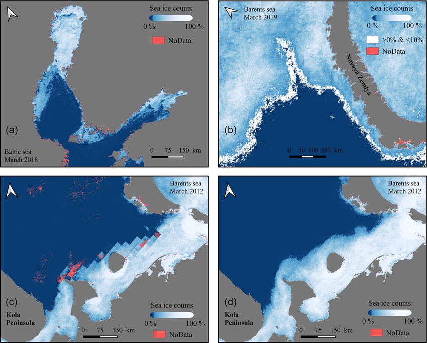
2804                                                     J. A. Parera-Portell et al.: Improved sea ice detection using MODIS

gional sea ice studies. On the other hand, active microwave
and visible-infrared sensors can acquire data at much higher
spatial resolutions. For instance, ESA’s satellites Sentinel-
1 (synthetic aperture radar) and Sentinel-2 (visible-infrared)
achieve resolutions of 5–100 m in the first case and 10–60 m
in the latter. However, such high-resolution sensors render
data with sparse spatial and temporal coverage due to their
small swath size and long revisit times, although this effect
is minimized at the poles. Instead, MODIS visible and in-
frared imagery offers a balanced trade-off between tempo-
ral and spatial coverage. MODIS is an imaging sensor on
board NASA’s sun-synchronous satellites Terra and Aqua,
launched in 1999 and 2002, respectively. It acquires data
in 36 spectral bands, ranging from the visible spectrum to
the thermal infrared. Spatial resolution at nadir varies from
250 m (bands 1 and 2) to 500 m (bands 3–7) and 1 km (bands
8–36) and has a large swath width of 2330 km. The MODIS
Terra and Aqua MOD29 and MYD29 datasets (Hall et al.,
2015a, b) provide daily global sea ice extent coverage at 1 km
but frequently fail to map the sea ice edge at this level of de-
tail. This is caused by the MODIS MOD35_L2 cloud mask              Figure 1. Northern European regional seas, as defined by the
product (Ackerman et al., 2010; MODIS Atmosphere Sci-              MSFD: (1) Iceland Sea, (2) Norwegian Sea, (3) Barents Sea, (4)
ence Team, 2017), the accuracy of which depends on the cor-        White Sea, (5) Baltic Sea, (6) Greater North Sea, and (7) Celtic
                                                                   Seas. In medium blue are shown the target sea regions, whereas in
rect identification of background sea ice at 25 km resolution
                                                                   light blue is the generated buffer, whose external limit corresponds
(Riggs and Hall, 2015). Therefore, sea ice beyond this back-       to the total processed area. All maps in this work are shown in North
ground is finally labelled as cloud instead of clear, eventually   Pole Lambert azimuthal equal area.
preventing the products which rely on this cloud mask from
accurately mapping the sea ice cover.
   In this context, a new 500 m resolution MODIS sea ice de-       2     Materials and methods
tection algorithm (IceMap500) was developed, aiming at the
improvement of existing European sea ice extent indicators         2.1    Study area
based on passive microwave observations (EEA, 2020) by
providing additional and higher-resolution data. IceMap500         This work focuses on the European regional seas established
is heavily influenced by the cloud masking and classification      by the MSFD (EEA, 2018). As sea ice only occurs in the
approaches of the previous IceMap250 algorithm (Gignac             northernmost oceanic sea regions or in enclosed, low-salinity
et al., 2017), which nonetheless is still vulnerable to the        water bodies such as the Baltic Sea, spatial coverage has been
MOD35_L2 background effects. The new algorithm is op-              significantly reduced to avoid the processing of uninforma-
timized to minimize classification errors and improves the         tive data. The final study area extends over the sea regions
quality of the maps by introducing a five-step workflow to         in Fig. 1, covering an area of roughly 4 ×10⁶ km2 . With the
prevent MOD35_L2 from breaking the 500 m resolution.               inclusion of a 400 km buffer to coherently join all the tar-
   To test the usefulness of IceMap500 as a European sea           get regional seas in a single study region, the totality of the
ice extent indicator, we analyse the sea ice trends in the         processed area sums up to approximately 8 ×10⁶ km2 .
European regional seas from 2000 to 2019 using MODIS                  Oceanic sea ice in the Northern Hemisphere has both a
Terra data. The analysis covers the northernmost European          perennial and a seasonal fraction. Typically, maximum and
sea regions defined by the European Union’s Marine Strat-          minimum sea ice extent are reached in March and September
egy Framework Directive (MSFD) where sea ice might oc-             (e.g. Stroeve et al., 2008), respectively, with the perennial
cur (EEA, 2018) and is restricted to the months when the           fraction being mostly enclosed in the Arctic basin (Comiso,
maximum and minimum sea ice extents are reached in the             2009). The ice cover in the Baltic Sea, however, has no peren-
Northern Hemisphere, that is, March and September, respec-         nial fraction and can be highly variable due to the milder
tively.                                                            climate, often resulting in different freezing and melting pe-
                                                                   riods during the same winter (Granskog et al., 2006). The sea
                                                                   ice season usually lasts for 6 to 8 months, starting in October
                                                                   or November in the Bothnian Bay and the Gulf of Finland.
                                                                   Maximum extent is also normally reached in March (Haapala
                                                                   et al., 2015). Therefore, given the particular characteristics of

The Cryosphere, 15, 2803–2818, 2021                                                     https://doi.org/10.5194/tc-15-2803-2021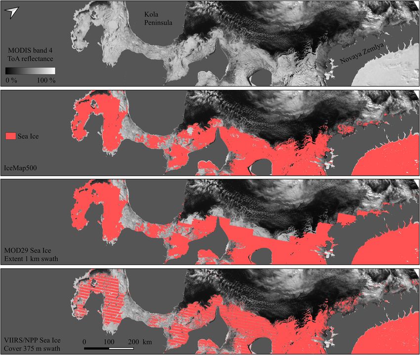
J. A. Parera-Portell et al.: Improved sea ice detection using MODIS                                                         2805

the Baltic Sea, the sea ice extent analysis is done by splitting
the study area in two regions: the NE Atlantic–Barents re-                    B4 − B2
gion (completely including the Iceland, Norwegian, Barents         NDSII2 =                                                   (2)
and White seas) and the Baltic region.                                        B4 + B2
                                                                      The VIS mask in IceMap250 is intended to identify areas
2.2   Selected data                                                where visibility is sufficient to perform a classification, for
                                                                   the sole goal of detecting open water. It uses the normalized
Data used in this work consist of MODIS Terra level 1B             difference between the MODIS thermal bands B20 and B32
top-of-atmosphere (ToA) radiance products MOD021KM                 as in Eq. (3).
(MODIS Science Team, 2017a), MOD02HKM (MODIS Sci-
ence Team, 2017b) and the MOD35_L2 cloud mask (MODIS                              B20 − B32
Atmosphere Science Team, 2017), as summarized in Table 1.          R(B20/B32) =                                               (3)
                                                                                  B20 + B32
Swath data are resampled to 500 m resolution if necessary,
converted to GeoTIFF format and projected to North Pole               The standard score of R(B20/B32) is then calculated, as seen
Lambert azimuthal equal area using HDF-EOS to GeoTIFF              in Eq. (4), where µ and σ are the mean and standard devia-
Conversion Tool (HEG) v2.15 (NASA, 2019). No stitching             tion of R(B20/B32) of the swath data to be classified. Pixels
is applied, as each scene is processed individually. How-          where VIS < 0.5 are tagged as having enough visibility. The
ever, scenes are clipped according to the selected study area.     masking produces the MOD35 and the VIS datasets, which
IceMap500 uses ToA radiance as input data, which are later         are classified separately and later combined following the set
converted to ToA reflectance or ToA brightness temperature,        of rules in Table 2.
so there is no atmospheric correction. Note that the objective             R(B20/B32) − µ
of the algorithm is to map sea ice presence rather than using      VIS =                                                      (4)
                                                                                 σ
reflectance as a proxy to get other physical variables such
as sea ice concentration, so the absence of atmospheric cor-          Although masking in IceMap250 is done at a resolution of
rection reduces processing time, facilitates the algorithm’s       1 km, the algorithm maps sea ice and water at 250 m within
replicability and ensures the consistency of the dataset.          the masked area. This is accomplished by means of a down-
                                                                   scaling technique by Trishchenko et al. (2006).
2.3   Overview of previous MODIS sea ice extent
      algorithms                                                   2.4   IceMap500: challenges and improvements

IceMap500 is fundamentally based on the previous IceMap            Both IceMap and IceMap250 face some challenging limita-
(Riggs et al., 1999; Hall et al., 2001) and IceMap250 (Gignac      tions which IceMap500 tries to address. The most important
et al., 2017) algorithms and inherits many of their features.      issue arises from the MOD35_L2 cloud mask, as it occasion-
Both algorithms feature a classification strategy based on         ally features resolution-breaking square artefacts of 25 km
threshold tests but differ on the cloud masking approach.          side length along the ice edge (Fig. 2) that prevent its ac-
IceMap uses the Normalized Difference Snow Index (NDSI,            curate mapping. Such artefacts originate in the setting of the
Eq. 1) as the main criterion to classify sea ice, followed by a    snow/ice background flag during the production process of
ToA threshold test using MODIS B4 (545–565 nm). To pre-            the mask (Riggs and Hall, 2015), in which NSIDC’s Near-
vent misclassification of clouds as sea ice, this algorithm uses   real-time Ice and Snow Extent (NISE) product (Brodzik and
the MOD35_L2 cloud mask as an input and outputs sea ice            Stewart, 2016), based on SSM/I-SSMIS passive microwave
extent at 1 km resolution.                                         data with a cell size of 25 km, is used to determine the flag’s
                                                                   state. Therefore, as the cloud detection algorithm takes dif-
         B4 − B6                                                   ferent paths depending on the background flag, sea ice falling
NDSI =                                                      (1)
         B4 + B6                                                   outside the footprint of the NISE classification is ultimately
                                                                   tagged as cloud in MOD35_L2. These 25 km artefacts can
  Instead, IceMap250 uses the Normalized Difference Snow
                                                                   occupy extensive areas in some scenes, causing the loss of
and Ice Index 2 (NDSII-2, Eq. 2) (Keshri et al., 2009), as
                                                                   many cloud-free classifiable pixels.
well as the same ToA reflectance threshold at 545–565 nm
                                                                      Another notable source of classification errors, this time
to classify sea ice and water. The threshold value of the
                                                                   only in IceMap250, arises from the NDSII-2 test, which uses
NDSII-2 is determined by splitting data in two groups with a
                                                                   the Jenks natural breaks optimization to split pixels in two
Jenks natural breaks optimization (Jenks, 1967), which max-
                                                                   groups, regardless of the surface classes present in a scene.
imizes inter-class variance and minimizes intra-class vari-
                                                                   When batch processing MODIS data it may be likely to run
ance. This algorithm features a hybrid cloud masking ap-
                                                                   into scenes lacking either ocean water or sea ice, and, con-
proach designed to minimize error while maximizing the
                                                                   sequently, the Jenks optimization splits pixels into both sur-
mapped area, using the MOD35_L2 cloud mask alongside
                                                                   face classes erroneously. Clouds that are undetected by the
an additional visibility (VIS) mask, both at 1 km resolution.
                                                                   MOD35_L2 cloud mask algorithm (Ackerman et al., 2010)

https://doi.org/10.5194/tc-15-2803-2021                                                 The Cryosphere, 15, 2803–2818, 2021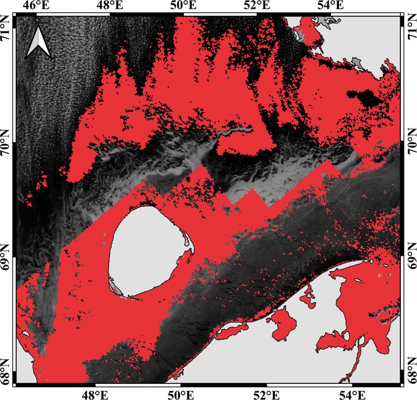
2806 J. A. Parera-Portell et al.: Improved sea ice detection using MODIS
Table 1. MODIS Terra swath data used in this work. Accessible at NASA’s Level-1 and Atmosphere Archive (https://ladsweb.modaps.eosdis.
nasa.gov, last access: 26 April 2021).
Band Bandwidth Spectrum region Code
MOD02HKM (bands 1–7 at 500 m resolution)
2 841–876 nm Near-infrared (NIR) B2
4 545–565 nm Green (G) B4
7 2.105–2.155 µm Short-wavelength infrared (SWIR) B7
MOD021KM (bands 8–36 at 1 km resolution)
20 3.660–3.840 µm Mid-wavelength infrared (MWIR) B20
32 11.770–12.270 µm Thermal infrared (TIR) B32
MOD35_L2 (cloud mask product)
Table 2. IceMap250 possible combinations of the classified maps and sun glint over ocean water may also be common error
and corresponding outputs (Gignac et al., 2017). sources due to the similar reflectance characteristics to sea
ice, in both IceMap and IceMap250. Additionally, as stated
MOD35 map VIS map Composite map in Gignac et al. (2017), bare ice and melt ponds may also fail
Ice ice ice the classification tests due to the similarity with ocean water.
Ice water water To mitigate those potential classification errors,
Ice NoData NoData IceMap500 features changes in the data masking and
Water ice NoData the classification rules. The new algorithm uses the dual
Water water water masking approach and the NDSII-2 and B4 ToA reflectance
Water NoData NoData tests as IceMap250 but increases the restrictiveness of
NoData ice NoData the masking and the classification. It also introduces an
NoData water water additional sea surface temperature (SST) test and a new
MOD35 correction workflow to minimize the effect of
the NISE footprint and enlarge the mapped area (see the
structure in Fig. 3). The downscaling technique used in
IceMap250 is not applied for various reasons: (I) simplicity,
(II) reduced processing times, (III) MODIS Aqua band
to band registration errors which may be even larger than
the 250 m cell size itself (Xiong et al., 2006; Khlopenkov
and Trishchenko, 2008), and (IV) spectral integrity of the
imagery (since no downscaling is applied). IceMap500
swath maps can be aggregated at any desired timescale.
We use a map aggregation approach which is sensitive
to spatio-temporal variations in sea ice and which can be
used to filter out unreliable sea ice classifications. The next
sections give a more in-depth explanation of the IceMap500
workflow.
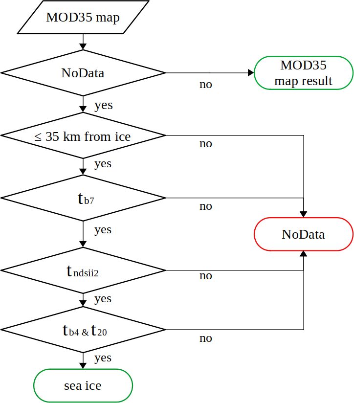
2.4.1 The masking
IceMap500 uses the same hybrid cloud masking approach
as IceMap250. The VIS mask is used and calculated as
in IceMap250, using the same VIS < 0.5 threshold value.
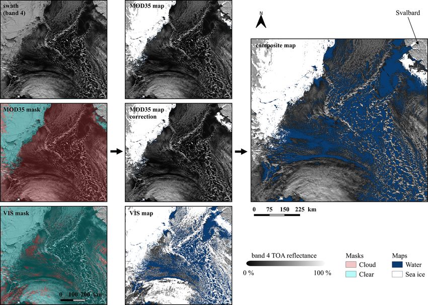
Figure 2. Pixels tagged as confident clear in the MOD35_L2 cloud Therefore, IceMap500 also generates the MOD35 and the
mask, shown in red, overlaying MODIS B4 swath data from March VIS datasets. Nevertheless, the MOD35 mask includes ad-
2012 (Barents sea). The footprint left by NISE on the cloud mask ditional constraints so not only cloud cover is considered
can be clearly seen along the ice edge. but also the lighting conditions, sun glint and presence of
land. This information is contained within the MODIS prod-
uct MOD35_L2, which provides multiple quality assessment
The Cryosphere, 15, 2803–2818, 2021 https://doi.org/10.5194/tc-15-2803-2021
J. A. Parera-Portell et al.: Improved sea ice detection using MODIS                                                         2807

                                                                       (Eq. 2) with the Jenks natural breaks optimization. Pix-
                                                                       els in the first group (i.e. NDSII-2 < k) are classified
                                                                       as sea ice. This test was shown to discriminate 96 %–
                                                                       100 % of sea ice even during the melting periods in
                                                                       Gignac et al. (2017).

                                                                   2. Green ToA reflectance test (tb4 ). Same as in both
                                                                      IceMap and IceMap250. A pixel is tagged as sea ice
                                                                      if its reflectance is > 17 % at 545–565 nm (B4). This
                                                                      threshold is based on the contrast in reflectance be-
                                                                      tween ice and water at visible wavelengths and was first
                                                                      used in Riggs et al. (1999) and later validated in Gignac
                                                                      et al. (2017). Gignac et al. (2017) demonstrated that a
                                                                      B4 > 17 % threshold resides slightly into the upper stan-
                                                                      dard deviation of the water class reflectance, so the risk
                                                                      of misclassifying melt ponds, leads, polynyas and low-
                                                                      albedo sea ice is low.

                                                                   3. Mid-range infrared temperature test (tb20 ). This new
                                                                      threshold is based on the sea surface temperature (SST)
                                                                      using B20 (3.660–3.840 µm). It is always used in con-
                                                                      junction with tb4 , although only in the MOD35 dataset
                                                                      classification. Therefore, sea ice is classified only when
                                                                      both B4 > 17 % and SST < 1 ◦ C. The tb20 test is used as
Figure 3. Simplified structure of IceMap500.                          a sort of mask to confirm that a pixel tagged as sea ice
                                                                      really belongs to sea ice, as unmasked sun glint, turbid
                                                                      water and aerosols may raise water reflectance past the
flags (Strabala, 2004; Ackerman et al., 2010). We use the fol-        tb4 threshold. To perform this test B20 is temporarily at-
lowing flag states:                                                   mospherically corrected with a straightforward equation
  1. Unobstructed FOV selects only pixels identified as con-          used in the MODIS SST algorithm (Brown and Minnett,
     fident clear, with a confidence of 99 % (Ackerman et al.,        1999) for mid-range infrared SST derivation (Eq. 5):
     2010).
                                                                       SST = 1.01342 + 1.04948TB20 ,                          (5)
  2. Day/Night selects only pixels identified as day. This flag
     is of special importance during the winter months, when           where TB20 is the brightness temperature of B20. The
     the polar twilight zone reaches the lowest latitudes, and,        1 ◦ C threshold is designed to include leads, cold wa-
     therefore, the available daytime area becomes scarcer.            ter, new sea ice and melt ponds (which according to
                                                                       Zhang et al. (2017) typically stay below 0.3 ◦ C) to
  3. Sun glint selects only pixels identified as no sun glint.         prevent breaking the 500 m resolution, while still dis-
     This way, areas with sun glint caused by the reflec-              carding most open water (refer, for instance, to global
     tion angle of the sun being between 0 and 36◦ are dis-            SST products such as NOAA High Resolution SST
     carded. Other potential sun glint sources are not consid-         by NOAA/OAR/ESRL PSL, Boulder, Colorado, USA,
     ered (Ackerman et al., 2010).                                     available at https://psl.noaa.gov/data/gridded/data.noaa.
                                                                       oisst.v2.highres.html, last access: 26 April 2021). More-
  4. Land/Water selects only pixels identified as water. Land
                                                                       over, B20 may be contaminated by reflected solar radia-
     masking is crucial to ensure the quality of the resulting
                                                                       tion, causing TB20 to increase and therefore making the
     classification because, as already pointed out in Gignac
                                                                       exclusion of sun glint easier.
     et al. (2017), an incorrect masking may generate sea ice
     false positives due to the reflectance contrast of land         In addition, IceMap500 features restrictive classification
     with water.                                                  rules to compensate for the output of tndsii2 in scenes with a
                                                                  single surface class, as the Jenks optimization will still split
2.4.2   The classification tests
                                                                  data into two groups. The classification rules depend on the
In IceMap500 three different threshold tests are included.        dataset that is being classified, as when merging the MOD35
                                                                  and VIS maps changes in a single dataset classification, ulti-
  1. NDSII-2 test (tndsii2 ). Same as in IceMap250. The           mately affecting the whole outcome. The classification rules
     threshold value k is determined by slicing the NDSII-2       are shown in Table 3: sea ice is only mapped in the MOD35

https://doi.org/10.5194/tc-15-2803-2021                                                The Cryosphere, 15, 2803–2818, 2021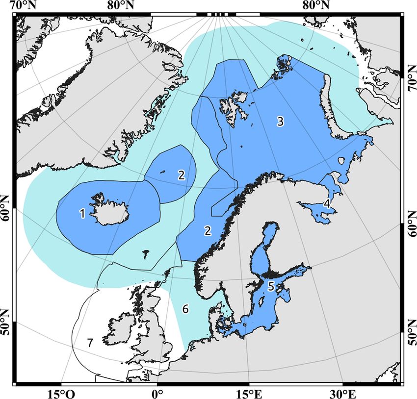
2808                                                     J. A. Parera-Portell et al.: Improved sea ice detection using MODIS

dataset when there is consensus between the tests, while in
the VIS dataset it is mapped whenever tb4 is positive. A
downside of this method is that it may leave some melt ponds
as NoData, since in the most advanced melting states they
tend to show NDSII-2 values similar to water (Gignac et al.,
2017). Note that while masking is done at 1 km resolution,
the swath data that are classified are at 500 m, so sea ice and
water are mapped at 500 m within the mask limits.

2.4.3   MOD35 correction

Once the MOD35 map is created, an additional set of tests
is introduced to attenuate the effects of the NISE foot-
print present in the MOD35_L2 mask, which propagate to
the MOD35 classification and ultimately to the composite
maps. Although the inclusion of this correction increases the
chances of classification errors, it greatly improves the sea
ice edge delineation and increases the classified area. The
MOD35 correction is designed to reclassify NoData pixels
within a buffer zone surrounding clusters of sea ice. Within
this buffer the MOD35_L2 cloud mask is ignored during              Figure 4. MOD35 block correction structure and possible test out-
the classification. Instead, MODIS B7 (2.105–2.155 µm) is          comes.
used to detect clear areas by taking advantage of the very
low reflectance values that water, snow and ice display at
such wavelengths, allowing cloud discrimination (e.g. Plat-                pling, although most of the remaining samples belong
nick et al., 2001; Thompson et al., 2015). To avoid error am-              to sea ice far from the ice edge, which is of no interest
plification, sea ice clusters below 100 pixels are deleted be-             in the MOD35 correction. However, by setting such a
fore the correction: if those clusters are found far from the              restrictive threshold only a small fraction of clouds are
ice edge, it is likely that they originate from sun glint or un-           included (1.5 %), which is preferred over including all
masked clouds, while those found close to large clusters of                sea ice while increasing sea ice false positives due to the
sea ice are ultimately classified again as such. The MOD35                 cloud cover.
correction includes five tests, as illustrated in Fig. 4.            4. tndsii2 . They are the same as in the MOD35 classifica-
                                                                        tion. Pixels where NDSII-2 < k pass the test, otherwise
 1. NoData test. NoData pixels pass the test, while classi-
                                                                        they are set as NoData. In this case, the Jenks optimiza-
    fied areas remain the same. All pixels set as NoData dur-
                                                                        tion is not performed using all the clear pixels in the
    ing the MOD35 classification also undergo the tests and
                                                                        scene but rather only those within the 35 km buffer zone
    may finally be labelled as sea ice or water.
                                                                        set as clear by tb7 .
 2. Euclidean distance test. NoData pixels found at 35 km            5. tb4 and tb20 . They are the same as in the MOD35 clas-
    or closer to a cluster of sea ice pass the test; otherwise          sification. Pixels where B4 > 17 % and SST < 1 ◦ C are
    they are set as NoData. This distance is roughly equal              classified as sea ice, otherwise they are set as NoData.
    to the diagonal of NISE’s 25 km cells and is used to re-
    duce the chances of misclassifying clouds as sea ice by           Finally, the MOD35 map and the result of the MOD35
    setting a buffer along the ice edge.                           block correction are merged and later combined with the VIS
                                                                   map according to the compositing rules in Table 2. A visual
 3. Short-wavelength infrared ToA reflectance test (tb7 ).         example of the workflow in IceMap500 is given in Fig. 6,
    Pixels below 3.5 % ToA reflectance at 2.105–2.155 µm           illustrating each intermediate result of the algorithm.
    (B7) pass the test, otherwise they are set as NoData.
    This threshold is based on the low reflectance that water,     2.4.4     Map aggregation and calculation of sea ice extent
    snow and ice display around 2 µm: spectral signatures in
    Fig. 5 indicate a maximum reflectance of ∼ 10 % for ice        The corrected MOD35 and VIS maps created for each scene
    within the B7 bandwidth, while the reflectance of snow         are combined to take advantage of the strengths of both the
    and water is always below 5 %. This test is used as a          MOD35 and the VIS classification methods, following the
    cloud filter, as it is expected that clouds show higher        criteria seen in Table 2. The extensive cloud cover found in
    reflectance values. Figure 5 also shows the threshold in-      most scenes and the restrictiveness of the classification im-
    cludes only 45.3 % of clear areas according to our sam-        ply that only a small area is finally mapped, although the

The Cryosphere, 15, 2803–2818, 2021                                                      https://doi.org/10.5194/tc-15-2803-2021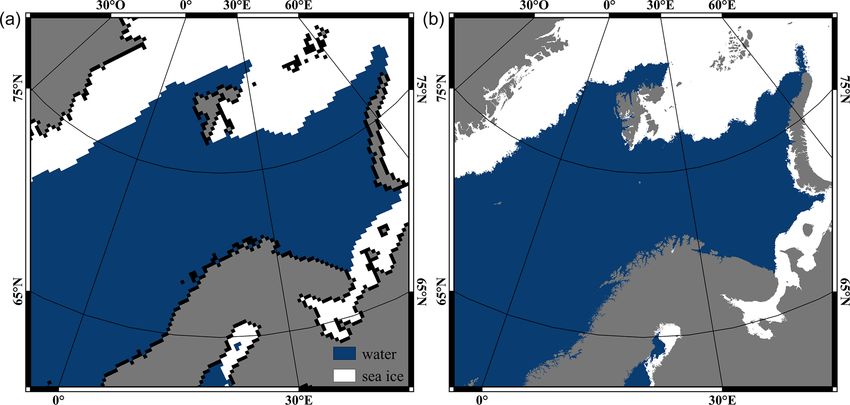
J. A. Parera-Portell et al.: Improved sea ice detection using MODIS                                                                      2809

Table 3. Classification outcomes based on the threshold tests in IceMap500.

                                            MOD35 dataset                                 VIS dataset
                                            tb4 >17 %
                              tndsii2 < k                  MOD35 map        tndsii2 < k    tb4 >17 %    VIS map
                                            tb20 < 1 ◦ C
                              Yes           yes            ice              yes            yes          ice
                              Yes           no             NoData           yes            no           NoData
                              No            yes            NoData           no             yes          ice
                              No            no             water            no             no           water

Figure 5. (a) Spectral signatures of several surfaces obtained from the USGS spectral library (Kokaly et al., 2017), including ice (frost), sea
water (oceanic and coastal) and snow-slush at different melting states (indicated by roman numerals); MODIS band 7 bandwidth is shown
in yellow. (b) Histograms for pixels identified as confident clear and other (probably clear, uncertain clear and cloudy) in the MOD35_L2
product, from 8000 randomly sampled points on five different scenes. Percentages indicate the proportion of pixels inside each filled area
using a 3.5 % ToA reflectance threshold.

new correction reduces the impact of the cloud mask. In any               able enough. By eliminating such observations, a small No-
case, many scenes are required to map large expanses of the               Data buffer zone along the ice edge is generated. IceMap500
sea ice cover. In IceMap500 a map aggregation method based                then takes advantage of the pixels set as water and fills the
on the number of coincident sea ice classifications achieved              NoData gaps using a Euclidean distance allocation method.
in each pixel is used, meaning that pixels classified as sea              This way a clearer and smoother sea ice edge is obtained,
ice in a large number of scenes will have higher reliability.             which nonetheless does not ignore the information carried
The aggregated maps are generated by calculating the sum of               by pixels where likelihood falls below the selected threshold.
composite maps where ice = 1 and water = 0 and later nor-                 This procedure acts as an additional post-classification error
malizing the results according to the maximum number of                   filter and produces a sea ice extent map, as the constant mo-
coincident sea ice observations achieved. With MODIS Terra                tion of the ice tends to hide the presence of features such as
the maximum number of observations typically reaches ∼ 50                 leads, cracks, polynyas and ice floes.
in March and ∼ 60 in September, so using both Terra and                       It is worth noting that the aggregation procedure eventu-
Aqua, this number could double and significantly increase                 ally sets either NoData pixels that were never really classi-
the usefulness of this method. The output provides informa-               fied by the algorithm during the entire time period as sea ice
tion about where sea ice is more likely to be found; thus we              or water. Although the dual masking approach and the use
appropriately refer to the resulting maps as sea ice presence             of the MOD35 correction greatly improve the final classified
likelihood maps (Fig. 7). This approach allows users to de-               area, NoData gaps still tend to appear in the regions closer to
tect the places where sea ice has been more unstable during               the pole in the March monthly maps as a consequence of the
a given time period, as the sea ice presence likelihood will              poor lighting conditions. This also makes sea ice presence
drop in such cases. Likelihood maps even allow the detection              likelihood to drop. September has no such lighting limita-
of cracks in the sea ice, and of course if sea ice has moved              tions, so NoData gaps appear more randomly. Fortunately,
significantly the sea ice presence likelihood will be lower.              the average NoData area fraction of our monthly time series
   Sea ice extent is obtained from the likelihood maps by se-             only reaches 1.0 % in March and 0.7 % in September.
lecting a likelihood threshold, in this case 10 %. Then, pixels
where sea ice presence is > 0 % and < 10 % (0 % is water)
are discarded because such observations might not be reli-

https://doi.org/10.5194/tc-15-2803-2021                                                           The Cryosphere, 15, 2803–2818, 2021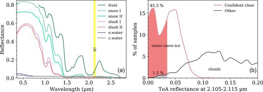
2810                                                      J. A. Parera-Portell et al.: Improved sea ice detection using MODIS

Figure 6. Intermediate and final products of IceMap500. The effect of the MOD35 correction is best seen on the upper right corner of the
maps.

3     Results                                                         sea ice cover. The resulting trend lines, represented in Fig. 8,
                                                                      have been obtained via least-squares linear regression.
We use the new IceMap500 algorithm to obtain swath and                   Results indicate that in the NE Atlantic–Barents region the
daily maps during the months of March and September of                sea ice decline is ∼ 70 % faster in March than in Septem-
the 2000–2019 period, using only MODIS Terra data. The                ber. Although September’s extent is comparatively smaller,
resulting maps have been aggregated at a monthly scale to             the standard error of the trends is similar in both months
obtain the time series of sea ice extent, from which sea ice          (∼ 6 × 10³ km2 yr−1 ), with R 2 being lower in September.
extent trends have been calculated. The performance of the            Nevertheless, both trends have been found to be statistically
algorithm is assessed with confusion matrices by manually             significant when considering a significance level of 99 %. In
validating swath maps.                                                particular, the March trend displays a very low p value, in-
                                                                      dicating a significance level of ∼ 99.98 %. In contrast, the
                                                                      Baltic Sea displays no clear tendency and a large variability.
3.1    Sea ice extent evolution and trends                            This causes R 2 to be very low and the standard error of the
                                                                      trend to be almost equal to the trend itself. If the 99 % signif-
Monthly sea ice extent maps have been used to determine               icance level criterion is followed, then H0 can not be rejected
the sea ice extent trends between 2000 and 2019 in the NE             in the Baltic Sea.
Atlantic–Barents region and the Baltic Sea separately. Both
March and September trends have been obtained for the NE              3.2   Accuracy assessment
Atlantic–Barents, that is, the trends of the maximum and
minimum sea ice cover, respectively. Since there is no peren-         We randomly selected 8 years to perform the quality assess-
nial sea ice fraction in the Baltic Sea, only the March trend         ment, from which a total number of 32 scenes have been
is available in this case, also corresponding to the maximum          used, that is, two scenes per month to allow comparison. As

The Cryosphere, 15, 2803–2818, 2021                                                        https://doi.org/10.5194/tc-15-2803-2021
J. A. Parera-Portell et al.: Improved sea ice detection using MODIS                                                                         2811

Figure 7. Clockwise from upper left: example of monthly sea ice presence likelihood in the Baltic Sea; buffer zone generated when setting
a 10 % likelihood threshold; monthly sea ice likelihood without MOD35 correction; monthly sea ice likelihood with MOD35 correction.

Figure 8. Monthly sea ice extent evolution and trend lines, alongside the numerical results of the sea ice trends and the standard error of the
slope. Two goodness-of-fit estimators are given: the coefficient of determination and the p value. P values are obtained from two-tailed Wald
tests with 18 degrees of freedom and null hypothesis that there is no correlation between the two variables, i.e. that the slope of the trend line
is zero.

https://doi.org/10.5194/tc-15-2803-2021                                                            The Cryosphere, 15, 2803–2818, 2021
2812                                                    J. A. Parera-Portell et al.: Improved sea ice detection using MODIS

a prerequisite, each validation scene must have both sea ice      tion is due to the misclassification of clouds as sea ice within
and water pixels. Validation has been carried out with con-       the limits of the sea ice cover; in fact, despite the cloud frac-
fusion matrices by generating 1500 random points per scene        tion being much larger over open ocean than over sea ice,
over the classified areas. Those points have been manually        in the first case sea ice commission errors are uncommon.
tagged as either sea ice, water or cloud, with the help of the    Some of the clouds that are commonly left undetected by
corresponding RGB swath. Although no clouds are mapped            the MOD35 cloud mask include low-level (top below 2 km),
in the algorithm, points found over clouds opaque enough to       high-level (top above 6 km) and thin clouds less than 2 km
avoid the identification of the surface below add to the total    thick (Chan and Comiso, 2013). Additionally, our validation
sea ice commission error.                                         showed that multilayered clouds cast shadows which can be
   Accuracy assessment results are summarized in Table 4.         finally tagged as sea ice. The rise of sea ice commission er-
All scenes achieved overall accuracies above 90 %, resulting      ror during September may be explained by the fact that, as
in an average accuracy of 96.0 %. The average kappa coeffi-       shown by Chan and Comiso (2013), late summer in the Arc-
cient of 0.85 indicates a strong agreement between classifica-    tic is considerably cloudier than winter, as lower sea ice con-
tion and ground truth, despite being affected by scenes with      centration relates to a larger cloud fraction.
few water validation points, causing the kappa coefficient to        Since sun glint issues have been mostly solved, as evi-
drop due to the disproportion between classes. Individually,      denced by the minimal impact of water omission error, and
only 5 out of 32 computed kappa coefficients are found be-        most sea ice commission is generated within the sea ice
low the 0.80 value, while 10 are found between 0.80–0.90          cover, there are few clusters of sea ice false positives over
and 17 above 0.90, indicating very strong agreement. The          open ocean, most of which are removed during the MOD35
primary source of error affecting the classification is sea ice   block correction. Thus, few of those errors are propagated to
commission, with its mean value alone adding up to 7.3 %,         the sea ice presence likelihood maps, allowing the selection
that is, more than sea ice omission, water commission and         of low threshold values to obtain sea ice extent.
water omission combined.
   By separately analysing both months, mean accuracy is          3.2.1   Agreement with NSIDC’s Sea Ice Index
found to be higher in March than September, differing by
1.9 %. Accuracy results in September are also slightly more       The Sea Ice Index (SII; Fetterer et al., 2017) is a widely
variable, showing a σ of 2.8 % versus 2.5 % in March. On the      used global sea ice extent and concentration product dis-
contrary, the mean kappa coefficient is lower in March than       tributed by the NSIDC, which is derived from satellite pas-
in September. This is linked to the much greater sea ice area     sive microwave data at 25 km spatial resolution. It covers
covered in March, which occasionally causes some scenes           from 1978 to the present, is updated on a daily basis and
to have very few water validation points, making the kappa        provides monthly median sea ice extent maps. In the Sea Ice
coefficient drop due to the disparity in validation points be-    Index (SII), extent is derived from sea ice concentration by
tween classes. The standard deviation of kappa greatly illus-     setting where concentration is 15 % or above as sea ice pix-
trates this issue, being 0.23 in March and 0.06 in September.     els. In spite of the difference in spatial resolution between
   Nevertheless, the difference in accuracy between months        the SII and IceMap500, measuring the agreement or simi-
does not arise from validation artefacts but mainly from          larity between both datasets can act as an estimator of the
the disparity in sea ice commission. With a mean sea ice          quality and consistency of IceMap500’s monthly aggregates.
commission error of 2.5 %, March classifications outperform       Thus, SII maps have been reprojected to North Pole Lambert
those for September, which show a mean error of 12.2 %.           azimuthal equal area and resampled down to a 500 m cell
Since there are only two classes, high water omission error       size. Then agreement has been calculated as the coincident
should be expected. However, it is very low in both cases,        sea ice area fraction between both datasets, compared to the
0.3 % in March and 0.04 % in September, revealing the dom-        total sea ice extent including coincident and non-coincident
inance of sea ice commission is not caused by the misclassi-      area (Eq. 6).
fication of water as sea ice but of clouds as sea ice. Instead,               T
sea ice omission error is similar in both months, being 2.7 %                A B
                                                                  Agreement = S ,                                              (6)
in March and 3.3 % in September, while water commission                      A B
is 2.5 % and 1.9 %, respectively. Thus, globally, the major er-
ror contribution is due to the misclassifications of clouds as    where A is an IceMap500 monthly aggregate and B the
sea ice, especially in September, while misclassification of      corresponding SII. Figure 9 illustrates the agreement for
sea ice as water and water as sea ice remain lower in the first   both March and September from 2000 to 2019. Mean agree-
case and minimal in the latter.                                   ment in March is 89.5 % with a standard deviation of 1.1 %,
   According to Chan and Comiso (2013), the MOD35_L2              whereas in September mean agreement is lower, 85.5 %,
cloud mask tends to underestimate the cloud cover over sea        and displays higher variability, with a standard deviation of
ice, whereas over open water it is overestimated but closer to    3.1 %. Only in a single case does the agreement fall below
reality. Indeed, most sea ice commission error in our valida-     80 %, corresponding to September 2013 (74.7 %).

The Cryosphere, 15, 2803–2818, 2021                                                   https://doi.org/10.5194/tc-15-2803-2021
J. A. Parera-Portell et al.: Improved sea ice detection using MODIS 2813
Table 4. Validation results for 32 swath maps. Two results are given per month, corresponding to different scenes. Commission (com.) and
omission (om.) errors represent the monthly mean. Kappa coefficients corresponding to scenes in which water validation points are less than
5 % from the total are shown in italics. The kappa statistic rates the agreement between classification and ground truth, although considering
that agreement may occur by chance (Cohen, 1960).
Accuracy (%) Kappa coefficient Sea ice com. / om. (%) Water com. / om. (%)
Year March September March September March September March September
2003 99.3, 97.9 94.0, 91.1 0.66, 0.88 0.88, 0.84 0.7 / 9.5 16.4 / 0.0 1.1 / 0.0 0.0 / 0.0
2005 95.3, 92.7 95.5, 99.1 0.95, 0.93 0.88, 0.97 0.0 / 6.2 10.2 / 2.1 5.4 / 0.0 0.4 / 0.0
2006 98.1, 98.6 94.1, 92.1 0.96, 0.97 0.88, 0.82 2.5 / 1.6 11.5 / 9.0 2.4 / 0.1 5.6 / 0.1
2008 97.4, 97.9 95.8, 98.0 0.94, 0.90 0.88, 0.95 2.2 / 1.0 11.6 / 1.3 2.8 / 0.0 0.4 / 0.0
2010 91.7, 97.8 90.8, 91.5 0.32, 0.96 0.83, 0.78 5.5 / 0.6 19.6 / 9.5 0.9 / 0.4 3.5 / 0.1
2011 98.3, 98.3 95.7, 98.6 0.96, 0.96 0.91, 0.97 0.4 / 2.0 3.9 / 2.1 4.8 / 0.1 2.9 / 0.1
2014 98.7, 99.1 92.4, 94.7 0.93, 0.98 0.84, 0.85 1.0 / 0.9 22.2 / 0.9 1.9 / 0.0 0.3 / 0.0
2016 93.7, 91.2 97.0, 99.2 0.32, 0.50 0.94, 0.98 7.8 / 0.0 1.8 / 1.5 0.7 / 2.1 1.9 / 0.0
Mean 96.9 95.0 0.82 0.89 2.5 / 2.7 12.2 / 3.3 2.5 / 0.3 1.9 / 0.0
Total
Mean 96.0 0.85 7.3 / 3.0 2.1 / 0.2
Median 97.2 0.91 4.7 / 1.5 1.9 / 0.0
considering a significance level of 99 %. The trends ob-
tained in this study are regional and therefore do not re-
flect the overall Arctic sea ice extent tendencies, although
they can be compared to studies in which regional trends
are also analysed. In Cavalieri and Parkinson (2012) the
summation of sea ice trends (1979–2010) in the Green-
land Sea and the Barents–Kara seas, roughly correspond-
ing to our study area, shows a greater loss of sea ice ex-
tent during winter (−21.7 ± 3.1 × 10³ km2 yr−1 ) than dur-
ing summer (−18.6 ± 3.2 × 10³ km2 yr−1 ). This is in accor-
dance with our results, and both trends are within the error
range of the trend lines in Fig. 8. Similarly, the summation
of the Greenland–Barents–Kara trends in Peng and Meier
(2017), covering from 1979 to 2015, indicates a trend of
Figure 9. Agreement between NSIDC’s Sea Ice Index and the ob- −19.0 ± 4.4 × 10³ km2 yr−1 for the maximum sea ice extent
tained monthly sea ice extent maps for all analysed years. and −14.9 ± 5.7 × 10³ km2 yr−1 for the minimum. This be-
haviour is also reported in the Barents Sea in Kumar et al.
(2021), spanning the 1979–2018 period. Nevertheless, the
An example of both datasets is shown in Fig. 10 for vi- sea ice extent loss is proportionally smaller in winter than
sual comparison: even though the difference in spatial res- in summer: in our study area the decadal sea ice loss is ap-
olution is not compensated for, both numerical and visual proximately 9 % in March and 13 % in September. Peng and
analyses suggest that IceMap500 monthly aggregates are co- Meier (2017) report sea ice losses of 10.1 % and 10.8 % per
herent with existing data even considering the different sea decade in the Greenland and Barents seas in winter, closely
ice extent calculation approach. matching our results.
In the case of the Baltic Sea, no statistically significant
trend can be inferred due to high interannual variability and
4 Discussion the limited lifespan of MODIS. This, however, does not im-
ply that H0 (i.e. that the Baltic ice cover is stable) is true:
4.1 Sea ice trends previous research (Jevrejeva et al., 2004) based on data from
coastal observatories covering the years 1900 to 2000 reveals
Sea ice trends obtained from our monthly extent maps in a significant decreasing trend in sea ice occurrence probabil-
the NE Atlantic–Barents region are consistent with previ- ity in the southern Baltic Sea, while in the northern half ice
ous observations, and both are statistically significant when
https://doi.org/10.5194/tc-15-2803-2021 The Cryosphere, 15, 2803–2818, 20212814 J. A. Parera-Portell et al.: Improved sea ice detection using MODIS
Figure 10. Comparison between NSIDC’s Sea Ice Index (a) and sea ice extent map obtained for March 2012 (b).
occurs every winter. Moreover, it shows a shortening of the resolution between both products. In the case of September
sea ice season and an advance in the date of break-up, es- 2013, the fragmentation of sea ice (notice the water pixels
pecially in the northern areas. More recent analyses (Vihma within the SII edge in Fig. 11) in combination with high sea
and Haapala, 2009; Haapala et al., 2015) also indicate that ice commission due to unmasked clouds led to an unusually
over the last century the sea ice season has shortened and low agreement score.
the occurrence of severe winters has fallen. Thus, although Overall, both the accuracy assessment of IceMap500 and
IceMap500 may not be suitable for Baltic sea ice monitoring the generally high agreement values with the SII suggest that
at a monthly scale due to the large variability, both interan- the new algorithm is well suited for sea ice studies and mon-
nually and within a same freezing period (Granskog et al., itoring. Its processing time also allows near-real-time map-
2006), it can be useful for detailed sea ice studies spanning ping: it takes around 50 min to generate a full daily map
shorter time periods. covering our study area (i.e. 16 scenes) using a modest ma-
chine with an Intel Xeon X5550 (4 × 2.67 GHz) processor
4.2 Applicability of IceMap500 and 12 GB RAM. Therefore, IceMap500 may represent an
improvement towards local and regional sea ice studies, es-
Accuracy assessment shows that the major source of error in pecially taking into account the spatio-temporal information
IceMap500 is sea ice commission, mostly caused by unde- carried by the sea ice presence likelihood maps. Additionally,
tected clouds. This is especially true in September due to the the inclusion of the MOD35 correction allows IceMap500 to
cloudier atmospheric conditions during the Arctic summer. map the sea ice edge more accurately than the MOD29 prod-
This issue is also reflected in the agreement with NSIDC’s uct (see the comparison in Fig. 12), which is visibly affected
SII, with the September agreement being lower than in by the NISE footprint. This increase in mapped area is also
March in all but 2 years and occasionally falling down to advantageous when aggregating maps at any timescale, as
75 % (September 2013). The larger number of scenes avail- sea ice presence likelihood rises and the presence of NoData
able during that month alongside the larger sea ice commis- gaps is minimized. Instead, in Fig. 12 the IceMap500 result
sion error make the September monthly aggregates poten- is closer in terms of both mapped area and spatial resolu-
tially affected by sea ice false positives to a greater extent, so tion to the VIIRS/NPP sea ice cover (375 m) swath product
a possible way of dealing with this situation is to increase the (Tschudi et al., 2017). It is worth noting, however, that VI-
sea ice presence likelihood threshold. In the case of Septem- IRS products may also be affected by the VIIRS cloud mask
ber 2013, a small change in the threshold value (from 10 % in the same way that MODIS is, because NISE is also used to
to 11 %) translates into an increase in IceMap500-SII agree- detect background sea ice in the VIIRS cloud mask algorithm
ment from 75 % to 80 % (see Fig. 11 for visual compari- (Frey et al., 2019).
son). An additional source of disagreement between SII and Even though IceMap500 is designed to work with
IceMap500 in the summer months is the greater fragmen- MODIS, it could also be used with other optical and infrared
tation of the ice cover, leading to the formation of sea ice sensors, as long as the selected sensor has equivalent bands to
floes, alongside the coastline discrepancy. However, these those used by this algorithm. Nevertheless, the application of
two sources are intrinsically linked to the difference in spatial the MOD35 correction, which would have to be adapted, de-
The Cryosphere, 15, 2803–2818, 2021 https://doi.org/10.5194/tc-15-2803-2021J. A. Parera-Portell et al.: Improved sea ice detection using MODIS 2815 Figure 11. Comparison between IceMap500 and the SII (September 2013) using two sea ice presence likelihood thresholds: 10 % (a) and 11 % (b). Figure 12. Comparison between IceMap500 swath composite, MOD29 sea ice extent and VIIRS/NPP sea ice cover products (26 March 2018). For MODIS Terra the swath acquisition time is 07:40 UTC, and for VIIRS/NPP it is 07:18 UTC. Disagreement between IceMap500 and MOD29 along the shoreline is attributed to land masking differences. https://doi.org/10.5194/tc-15-2803-2021 The Cryosphere, 15, 2803–2818, 2021
2816                                                     J. A. Parera-Portell et al.: Improved sea ice detection using MODIS

pends on the characteristics of the cloud mask to be used, and     Competing interests. The authors declare that they have no conflict
may not even be necessary. In the case of VIIRS the MOD35          of interest.
correction may be advantageous due to the potential effect
of the NISE background, but there is no direct equivalent
to MODIS B7, which is used to identify clouds during the           Acknowledgements. The authors thank the two anonymous referees
correction. Therefore, the potential of the closest match (VI-     and the editor Melody Sandells for their useful comments, which
IRS band M11, with a 2.20–2.30 µm bandwidth) to discern            greatly improved the manuscript. Work on software QGIS and the
                                                                   HDF-EOS to GeoTIFF Conversion Tool (HEG) is acknowledged.
clouds from the ice cover should be assessed in this con-
                                                                   Special thanks go to Jaume Fons-Esteve at the Department of Ge-
text. However, the application of the IceMap500 algorithm
                                                                   ography, Universitat Autònoma de Barcelona.
to both other sensors or other study regions might yield dif-
ferent accuracy assessment results, so the threshold tests or
the classification restrictiveness might need to be revised in     Review statement. This paper was edited by Melody Sandells and
each particular case to improve its performance.                   reviewed by two anonymous referees.

5   Conclusions
                                                                   References
The new IceMap500 algorithm is shown to generate high-
quality sea ice maps by systematically achieving accura-           Ackerman, S. A., Frey, R. A., Strabala, K., Liu, Y., Gumley, L. E.,
cies above 90 %. Quality assessment revealed the most                Baum, B., and Menzel, P.: Discriminating clear-sky from clouds
common error is sea ice commission caused by unmasked                with MODIS – Algorithm theoretical basis document, Tech.
                                                                     Rep., MODIS Cloud Mask Team and Cooperative Institute for
clouds, manifesting the key role that cloud masking plays
                                                                     Meteorological Satellite Studies, University of Wisconsin, Madi-
on the overall accuracy of the algorithm. The addition of the        son, USA, available at: https://modis-atmos.gsfc.nasa.gov/sites/
MOD35 correction substantially improves the delineation of           default/files/ModAtmo/MOD35_ATBD_Collection6_0.pdf (last
the ice edge, preventing the propagation of the NISE foot-           access: 8 October 2020), 2010.
print, and increases the mapped area, which is of capital im-      AMAP: Snow, Water, Ice and Permafrost, Summary for Policy-
portance when deriving daily and monthly maps due to the             makers, Tech. Rep., Arctic Monitoring and Assessment
restrictiveness of the classification and the weather depen-         Programme (AMAP), Oslo, Norway, available at: https://www.
dence of MODIS visible and infrared data. High agreement             amap.no/documents/doc/Snow-Water-Ice-and-Permafrost.
between our monthly sea ice extent maps and NSIDC’s Sea              -Summary-for-Policy-makers/1532 (last access: 8 October
Ice Index, especially in March, demonstrates the consistency         2020), 2017.
of the map aggregation method and further exemplifies the          Brodzik, M. J. and Stewart, J. S.: Near-Real-Time SSM/I-SSMIS
                                                                     EASE-Grid Daily Global Ice Concentration and Snow Extent,
overall good performance of the algorithm. Data produced
                                                                     Version 5 [Data set], NASA National Snow and Ice Data Cen-
by IceMap500 have proven useful to evaluate sea ice extent           ter Distributed Active Archive Center, Boulder, Colorado, USA,
trends in the NE Atlantic–Barents region and the Baltic Sea.         https://doi.org/10.5067/3KB2JPLFPK3R, 2016.
Significant negative trends have been observed in both March       Brown, O. B. and Minnett, P. J.: MODIS Infrared Sea Surface Tem-
and September in the NE Atlantic–Barents region, while the           perature Algorithm Theoretical Basis Document Version 2.0,
Baltic Sea displays much more variability, and no trend can          Tech. Rep., University of Miami, Florida, USA, available at:
be inferred from it. Given the high accuracies achieved and          https://modis.gsfc.nasa.gov/data/atbd/atbd_mod25.pdf (last ac-
the coherence with existing data, we find that IceMap500 is          cess: 8 October 2020), 1999.
a useful tool for sea ice studies and monitoring, particularly     Cavalieri, D. J. and Parkinson, C. L.: Arctic sea ice vari-
at local and regional scales.                                        ability and trends, 1979–2010, The Cryosphere, 6, 881–889,
                                                                     https://doi.org/10.5194/tc-6-881-2012, 2012.
                                                                   Chan, M. A. and Comiso, J. C.: Arctic Cloud Characteristics as De-
                                                                     rived from MODIS, CALIPSO, and CloudSat, J. Climate, 26,
Code and data availability. The source code is hosted at
                                                                     3285–3306, https://doi.org/10.1175/JCLI-D-12-00204.1, 2013.
https://doi.org/10.5281/zenodo.4973715 (Parera-Portell, 2021).
                                                                   Cohen, J.: A Coefficient of Agreement for Nom-
Monthly March and September sea ice extent maps from 2000 to
                                                                     inal    Scales,    Educ.    Psychol.    Meas.,      20,   37–46,
2019 are available at https://doi.org/10.5565/ddd.uab.cat/233396
                                                                     https://doi.org/10.1177/001316446002000104, 1960.
(Parera-Portell and Ubach, 2020).
                                                                   Collins, M., Knutti, R., Arblaster, J., Dufresne, J. L., Fichefet,
                                                                     T., Friedlingstein, P., Gao, X., Gutowski, W. J., Johns, T.,
                                                                     Krinner, G., Shongwe, M., Tebaldi, C., Weaver, A. J., and
Author contributions. RU and JAPP conceptualized the study.          Wehner, M.: Long-term Climate Change: Projections, Com-
JAPP developed the methodology and software, analysed the            mitments and Irreversibility, in: Climate Change 2013: The
dataset, and wrote the original draft. RU and CG supervised re-      Physical Science Basis, Contribution of Working Group I to
search and reviewed and edited the manuscript.                       the Fifth Assessment Report of the Intergovernmental Panel
                                                                     on Climate Change, edited by: Stocker, T. F., Qin, D., Plat-

The Cryosphere, 15, 2803–2818, 2021                                                    https://doi.org/10.5194/tc-15-2803-2021
J. A. Parera-Portell et al.: Improved sea ice detection using MODIS 2817 tner, G.-K., Tignor, M. M. B., Allen, S. K., Boschung, J., Jenks, G. F.: The data model concept in statistical mapping, in: In- Nauels, A., Xia, Y., Bex, V., and Midgley, P. M., p. 1535, ternational Yearbook of Cartography, edited by: Frenzel, K., Ber- Cambridge University Press, Cambridge, UK, New York, USA, telsmann Verlag, Gütersloh, Germany, 186–190, 1967. available at: http://www.climatechange2013.org/images/report/ Jevrejeva, S., Drabkin, V. V., Kostjukov, J., Lebedev, A. A., Lep- WG1AR5_Chapter12_FINAL.pdf (last access: 8 October 2020), päranta, M., Mironov, Y. U., Schmelzer, N., and Sztobryn, M.: 2013. Baltic Sea ice seasons in the twentieth century, Climate Res., 25, Comiso, J. C.: Variability and Trends of the Global Sea 217–227, https://doi.org/10.3354/cr025217, 2004. Ice Cover, in: Sea Ice, edited by: Thomas, D. N. and Keshri, A. K., Shukla, A., and Gupta, R. P.: ASTER ratio indices for Dieckmann, G. S., Wiley-Blackwell, Oxford, UK, 205–246, supraglacial terrain mapping, Int. J. Remote Sens., 30, 519–524, https://doi.org/10.1002/9781444317145.ch6, 2009. https://doi.org/10.1080/01431160802385459, 2009. Comiso, J. C., Meier, W. N., and Gersten, R.: Variability and Khlopenkov, K. V. and Trishchenko, A. P.: Implementation and trends in the Arctic Sea ice cover: Results from differ- Evaluation of Concurrent Gradient Search Method for Reprojec- ent techniques, J. Geophys. Res.-Oceans, 122, 6883–6900, tion of MODIS Level 1B Imagery, IEEE T. Geosci. Remote, 46, https://doi.org/10.1002/2017jc012768, 2017. 2016–2027, https://doi.org/10.1109/TGRS.2008.916633, 2008. EEA: MSFD Europe Seas, version 1, available at: https://www.eea. Kokaly, R. F., Clark, R. N., Swayze, G. A., Livo, K. E., Hoefen, europa.eu/data-and-maps/data/europe-seas-1 (last access: 26 T. M., Pearson, N. C., Wise, R. A., Benzel, W. M., Lowers, H. A., April 2021), 2018. Driscoll, R. L., and Klein, A. J.: USGS Spectral Library Version EEA: Arctic and Baltic sea ice, Tech. Rep., European Environment 7, U.S. Geological Survey, Reston, VA, USA, U.S. Geological Agency, Copenhagen, Denmark, available at: https://www.eea. Survey Data Series 1035, 61 pp., https://doi.org/10.3133/ds1035, europa.eu/data-and-maps/indicators/arctic-sea-ice-2/assessment 2017. (last access: 26 April 2021), 2020. Kumar, A., Yadav, J., and Mohan, R.: Spatio-temporal change Fetterer, F., Knowles, K., Meier, W., Savoie, M., and Wind- and variability of Barents-Kara sea ice, in the Arctic: Ocean nagel, A.: Sea Ice Index, Version 3, NSIDC: National and atmospheric implications, Sci. Total Environ., 753, 142046, Snow and Ice Data Center, Boulder, Colorado, USA, https://doi.org/10.1016/j.scitotenv.2020.142046, 2021. https://doi.org/10.7265/n5k072f8, 2017. Kwok, R.: Arctic sea ice thickness, volume, and multiyear ice Frey, R. A., Ackerman, S. A., Holz, R. E., and Dutcher, S.: The coverage: losses and coupled variability (1958–2018), En- Continuity MODIS-VIIRS Cloud Mask (MVCM) User’s Guide, viron. Res. Lett., 13, 105005, https://doi.org/10.1088/1748- https://doi.org/10.3390/rs12203334, 2019. 9326/aae3ec, 2018. Gignac, C., Bernier, M., Chokmani, K., and Poulin, J.: IceMap250- Lindsay, R. and Schweiger, A.: Arctic sea ice thickness loss deter- Automatic 250 m Sea Ice Extent Mapping Using MODIS Data, mined using subsurface, aircraft, and satellite observations, The Remote Sens.-Basel, 9, 70, https://doi.org/10.3390/rs9010070, Cryosphere, 9, 269–283, https://doi.org/10.5194/tc-9-269-2015, 2017. 2015. Granskog, M. A., Kaartokallio, H., Kuosa, H., Thomas, Liu, Y., Key, J. R., Wang, X., and Tschudi, M.: Multidecadal Arc- D. N., and Vainio, J.: Sea ice in the Baltic Sea tic sea ice thickness and volume derived from ice age, The – A review, Estuar. Coast. Shelf S., 70, 145–160, Cryosphere, 14, 1325–1345, https://doi.org/10.5194/tc-14-1325- https://doi.org/10.1016/j.ecss.2006.06.001, 2006. 2020, 2020. Haapala, J. J., Ronkainen, I., Schmelzer, N., and Sztobryn, M.: Re- Massonnet, F., Fichefet, T., Goosse, H., Bitz, C. M., Philippon- cent Change-Sea Ice, in: Second Assessment of Climate Change Berthier, G., Holland, M. M., and Barriat, P.-Y.: Constraining for the Baltic Sea Basin, edited by: Bolle, H. J., Menenti, M., projections of summer Arctic sea ice, The Cryosphere, 6, 1383– Sebastiano, S., and Ichtiaque, S., Springer International Publish- 1394, https://doi.org/10.5194/tc-6-1383-2012, 2012. ing, Cham, Switzerland, 145–153, https://doi.org/10.1007/978- Meier, W., Hovelsrud, G. K., van Oort, B. E. H., Key, J. R., Ko- 3-319-16006-1_8, 2015. vacs, K. M., Michel, C., Haas, C., Granskog, M. A., Gerland, Hall, D. K., Riggs, G. A., Salomonson, V. V., Barton, J. S., Casey, S., Perovich, D. K., Makshtas, A., and Reist, J. D.: Arctic sea K. S., Chien, J. Y. L., DiGirolamo, N. E., Klein, A. G., Pow- ice in transformation: A review of recent observed changes and ell, H. W., and Tait, A. B.: Algorithm Theoretical Basis Docu- impacts on biology and human activity, Rev. Geophys., 52, 185– ment (ATBD) for the MODIS Snow and Sea Ice-Mapping Algo- 217, https://doi.org/10.1002/2013RG000431, 2014. rithms, Tech. Rep., NASA Goddard Space Flight Center, Green- MODIS Atmosphere Science Team: MODIS/Terra Cloud Mask and belt, Maryland, USA, available at: https://modis.gsfc.nasa.gov/ Spectral Test Results 5-Min L2 Swath 250 m and 1 km, NASA data/atbd/atbd_mod10.pdf (last access: 26 April 2021), 2001. MODIS Adaptive Processing System, Goddard Space Flight Hall, D. K., Riggs, G. A., Solomonson, V., and NASA MODAPS Center, USA, https://doi.org/10.5067/MODIS/MOD35_L2.061, SIPS: MODIS/Aqua Sea Ice Extent 5-Min L2 Swath 1 km 2017. [Data set], NASA National Snow and Ice Data Center Dis- MODIS Science Team: MOD021KM MODIS/Terra Calibrated tributed Active Archive Center, Boulder, Colorado, USA, Radiances 5-Min L1B Swath 1 km, NASA MODIS Adap- https://doi.org/10.5067/MODIS/MYD29.006, 2015a. tive Processing System, Goddard Space Flight Center, USA, Hall, D. K., Riggs, G. A., Solomonson, V., and NASA MODAPS https://doi.org/10.5067/MODIS/MOD021KM.061, 2017a. SIPS: MODIS/Terra Sea Ice Extent 5-Min L2 Swath 1 km MODIS Science Team: MOD02HKM MODIS/Terra Calibrated [Data set], NASA National Snow and Ice Data Center Dis- Radiances 5-Min L1B Swath 500 m, NASA MODIS Adap- tributed Active Archive Center, Boulder, Colorado, USA, tive Processing System, Goddard Space Flight Center, USA, https://doi.org/10.5067/MODIS/MOD29.006, 2015b. https://doi.org/10.5067/MODIS/MOD02HKM.061, 2017b. https://doi.org/10.5194/tc-15-2803-2021 The Cryosphere, 15, 2803–2818, 2021
You can also read