Current Large Marine Ecosystem - A monthly surface pCO2 product for the California - ESSD
←
→
Page content transcription
If your browser does not render page correctly, please read the page content below
Earth Syst. Sci. Data, 14, 2081–2108, 2022
https://doi.org/10.5194/essd-14-2081-2022
© Author(s) 2022. This work is distributed under
the Creative Commons Attribution 4.0 License.

             A monthly surface pCO2 product for the California
                    Current Large Marine Ecosystem
             Jonathan D. Sharp1,2 , Andrea J. Fassbender2 , Brendan R. Carter1,2 , Paige D. Lavin3,4 , and
                                                Adrienne J. Sutton2
          1 CooperativeInstitute for Climate, Ocean, and Ecosystem Studies (CICOES), University of Washington,
                                                    Seattle, WA 98195, USA
                    2 NOAA/OAR Pacific Marine Environmental Laboratory, Seattle, WA 98115, USA
          3 Cooperative Institute for Satellite Earth System Studies/Earth System Science Interdisciplinary Center

                         (CISESS/ESSIC), University of Maryland, College Park, MD 20740, USA
             4 NOAA/NESDIS Center for Satellite Applications and Research, College Park, MD 20740, USA

                             Correspondence: Jonathan D. Sharp (jonathan.sharp@noaa.gov)

                               Received: 30 September 2021 – Discussion started: 20 October 2021
                            Revised: 2 April 2022 – Accepted: 6 April 2022 – Published: 29 April 2022

      Abstract. A common strategy for calculating the direction and rate of carbon dioxide gas (CO2 ) exchange
      between the ocean and atmosphere relies on knowledge of the partial pressure of CO2 in surface seawater
      (pCO2(sw) ), a quantity that is frequently observed by autonomous sensors on ships and moored buoys, albeit
      with significant spatial and temporal gaps. Here we present a monthly gridded data product of pCO2(sw) at 0.25◦
      latitude by 0.25◦ longitude resolution in the northeastern Pacific Ocean, centered on the California Current Sys-
      tem (CCS) and spanning all months from January 1998 to December 2020. The data product (RFR-CCS; Sharp et
      al., 2022; https://doi.org/10.5281/zenodo.5523389) was created using observations from the most recent (2021)
      version of the Surface Ocean CO2 Atlas (Bakker et al., 2016). These observations were fit against a variety of
      collocated and contemporaneous satellite- and model-derived surface variables using a random forest regression
      (RFR) model. We validate RFR-CCS in multiple ways, including direct comparisons with observations from sen-
      sors on moored buoys, and find that the data product effectively captures seasonal pCO2(sw) cycles at nearshore
      sites. This result is notable because global gridded pCO2(sw) products do not capture local variability effectively
      in this region, suggesting that RFR-CCS is a better option than regional extractions from global products to
      represent pCO2(sw) in the CCS over the last 2 decades. Lessons learned from the construction of RFR-CCS pro-
      vide insight into how global pCO2(sw) products could effectively characterize seasonal variability in nearshore
      coastal environments. We briefly review the physical and biological processes – acting across a variety of spatial
      and temporal scales – that are responsible for the latitudinal and nearshore-to-offshore pCO2(sw) gradients seen
      in the RFR-CCS reconstruction of pCO2(sw) . RFR-CCS will be valuable for the validation of high-resolution
      models, the attribution of spatiotemporal carbonate system variability to physical and biological drivers, and the
      quantification of multiyear trends and interannual variability of ocean acidification.

Published by Copernicus Publications.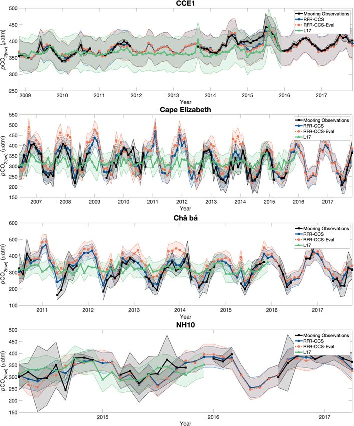
2082                                                            J. D. Sharp et al.: A monthly surface pCO2 product for the CCS

1   Introduction                                                     have become popular options as well (Gregor et al., 2019;
                                                                     Lebehot et al., 2019; Fay et al., 2021).
The concentration of carbon dioxide gas (CO2 ) in Earth’s                One widely used machine-learning-based pCO2(sw) gap-
atmosphere has rapidly increased from about 280 parts per            filling strategy relies on a two-step approach consisting of
million in 1750 to over 400 parts per million today (Joos            unsupervised clustering using a self-organizing-map (SOM)
and Spahni, 2008; Dlugokencky and Tans, 2019). This rise             followed by construction of a feed-forward neural network
in CO2 concentration is a direct result of human activities          (FFN) for each cluster (Landschützer et al., 2013). This
such as fossil fuel combustion, deforestation, and agriculture       SOM-FFN approach is well-established in the literature
(Ciais et al., 2014; Friedlingstein et al., 2020). The presence      (Landschützer et al., 2013, 2014, 2015, 2016, 2018; Laruelle
of human-produced or “anthropogenic” CO2 in the atmo-                et al., 2017; Ritter et al., 2017; Denvil-Sommer et al., 2019)
sphere – along with other anthropogenic greenhouse gases –           and is recognized as one of the most effective approaches
leads to planetary warming, with a disproportionate amount           for filling gaps in the observational pCO2(sw) record (Rö-
of heat (∼ 90 %) being absorbed by the ocean (von Schuck-            denbeck et al., 2015). The SOM-FFN approach was recently
mann et al., 2020). About a quarter of annually produced an-         applied to coastal ocean areas, resulting in the first globally
thropogenic CO2 dissolves directly into the ocean (Friedling-        continuous, multiyear data product of monthly coastal ocean
stein et al., 2020), mitigating its warming potential. How-          pCO2(sw) at 0.25◦ resolution (Laruelle et al., 2017). Even
ever, dissolved CO2 reacts with seawater to form carbonic            more recently, that coastal product was combined with an
acid, which rapidly dissociates and acidifies (primarily) sur-       updated open-ocean product (Landschützer et al., 2020a) to
face ocean environments (Caldeira and Wickett, 2003), with           produce a uniform 12-month climatology of pCO2(sw) across
adverse effects for many marine organisms and ecosystems             the coastal to open-ocean continuum (Landschützer et al.,
(Orr et al., 2005; Fabry et al., 2008; Pörtner, 2008; Doney et       2020b, c).
al., 2009, 2020). Closing the global carbon budget involves              The data products provided by Laruelle et al. (2017) and
accurately estimating the amount of CO2 taken up by the              Landschützer et al. (2020b) – hereafter L17 and L20, respec-
ocean (e.g., Hauck et al., 2020). A primary method for cal-          tively – are important advancements toward characterizing
culating the amount of CO2 transferred to the ocean requires         pCO2(sw) across the entire ocean domain for carbon budget
knowing the difference between the partial pressure of CO2           analyses. Most data-based estimates of oceanic CO2 uptake
in the atmosphere and surface seawater.                              have considered only the open ocean (e.g., Landschützer et
   Compared to atmospheric CO2 partial pressure                      al., 2014; Iida et al., 2015; Denvil-Sommer et al., 2019; Gre-
(pCO2(atm) ), which can be determined with some cer-                 gor et al., 2019; Watson et al., 2020) or are based on coarse
tainty at a given location even without direct observations          spatial representations of the coastal ocean (Rödenbeck et al.,
due to the well-mixed nature of the atmosphere, surface              2013). However, coastal ocean CO2 uptake is estimated to be
seawater CO2 partial pressure (pCO2(sw) ) is more variable           about 10 % of the open-ocean figure (Laruelle et al., 2010,
and therefore more difficult to constrain (Wanninkhof, 2014;         2014; Bourgeois et al., 2016; Roobaert et al., 2019; Chau et
Landschützer et al., 2014; Woolf et al., 2019). This variabil-       al., 2022), is far more spatially variable (Liu et al., 2010), and
ity is a result of ocean mixing, equilibration kinetics between      may be changing at a different rate relative to open-ocean
the atmosphere and ocean, biological processes, and thermal          CO2 uptake (Laruelle et al., 2018). Therefore, augmenting
effects on pCO2(sw) . Filling temporal and spatial data gaps         global open-ocean pCO2(sw) data products to include the
in the observational coverage of pCO2(sw) can therefore              coastal ocean is quite valuable (Fay et al., 2021). Despite
be challenging (Hauck et al., 2020; Fay et al., 2021) and            the greater spatial coverage and temporal resolution offered
a variety of strategies have been attempted over several             by these new gap-filled pCO2(sw) data products, significant
decades (Takahashi et al., 1993; Rödenbeck et al., 2015),            challenges remain for accurately representing pCO2(sw) .
becoming even more prevalent and varied in the literature                One of those challenges involves characterizing sea-
over time. Briefly, statistical interpolations (Takahashi et al.,    sonal cycles in pCO2(sw) , particularly in the nearshore
1993, 2002, 2009; Rödenbeck et al., 2013, 2014; Jones et             coastal ocean. Although the L17 product effectively captures
al., 2015; Shutler et al., 2016), multiple linear regressions        pCO2(sw) seasonality when averaged across relatively large
(Schuster et al., 2013; Iida et al., 2015; Becker et al., 2021),     coastal ocean regions, the authors assert that “the coastal
machine-learning-based regression methods (Landschützer              SOM-FFN tends to systematically underestimate the ampli-
et al., 2013; 2014, 2016, 2018; Nakaoka et al., 2013; Zeng           tude of the seasonal pCO2 cycle” in locations where they
et al., 2014; Laruelle et al., 2017; Ritter et al., 2017; Gregor     can make comparisons with direct observations. This result
et al., 2017, 2018; Chen et al., 2019; Denvil-Sommer et              is logical given that (1) direct observations are made at dis-
al., 2019), and biogeochemical-model-based approaches                crete locations and times, whereas gridded products are av-
(Valsala and Maksyutov, 2010; Majkut et al., 2014; Verdy             eraged over some spatial area and time, which tempers ex-
and Mazloff, 2017) have been common tactics, each one                tremes; and (2) fits obtained via least squares regressions
with its own strengths and weaknesses. Recently, ensemble            or machine-learning methods generally tend to perform bet-
averages of multiple data- or model-based approaches                 ter when temporal and spatial variability is low and worse

Earth Syst. Sci. Data, 14, 2081–2108, 2022                                            https://doi.org/10.5194/essd-14-2081-2022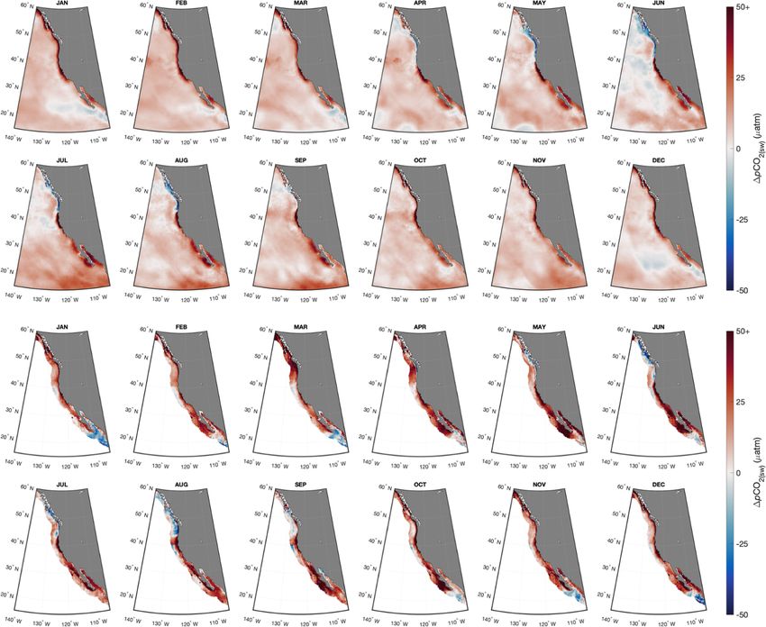
J. D. Sharp et al.: A monthly surface pCO2 product for the CCS                                                              2083

when variability is high (Landschützer et al., 2014), such        and over 1.4 million fCO2 (sw) observations within the study
as in the coastal ocean. However, this problem must be ad-        region.
dressed if we hope to achieve realistic global representations       SOCAT data in the study region were filtered to retain
of pCO2(sw) seasonality, which are necessary for investigat-      fCO2 (sw) observations with a measurement quality control
ing the processes that drive this variability (Roobaert et al.,   (QC) flag of 2 (“good”) and dataset QC flags of A through
2019) and for ensuring the fidelity of future air–sea CO2         D (fCO2 (sw) accuracy of 5 µatm or better). This is identical to
flux projections (Hauck et al., 2020). Addressing carbon ex-      the QC procedure followed by the SOCAT team for produc-
change in coastal margins has recently been highlighted as        ing gridded data products (Sabine et al., 2013; Bakker et al.,
a fundamental and emerging research topic in ocean carbon         2016). SOCATv2021 provides ancillary variables along with
research (Dai, 2021).                                             fCO2 (sw) , including contemporaneous observations of sea
    Here, we present a reconstruction of pCO2(sw) (1998–          surface temperature (SST) and sea surface salinity (SSS), as
2020) in a broad region of the northeastern Pacific that in-      well as atmospheric pressure at the ocean surface (Patm ) from
cludes the California Current System (CCS), the surrounding       the National Centers for Environmental Prediction (NCEP)
open-ocean regions, and the highly variable continental shelf     reanalysis; these values were used only for fugacity to partial
of the North American west coast spanning from southern           pressure conversions (Eq. 1). Though SST and SSS are con-
Alaska to Baja California. We apply a random forest regres-       sidered surface values, it is important to note that these are
sion (RFR) approach (Breiman, 2001) to fill observational         primarily underway measurements taken a few meters be-
gaps, constraining pCO2(sw) across the coastal to open-ocean      neath the surface and that nontrivial differences in tempera-
continuum. We show that the RFR approach in the north-            ture and salinity may exist between the measurement depth
eastern Pacific produces realistic monthly maps of surface        and the surface (Robertson and Watson, 1992; Donlon et al.,
pCO2(sw) from 1998 to 2020 and that these maps reliably           2002; Goddijn-Murphy et al., 2015; Woolf et al., 2016; Ho
capture seasonal pCO2(sw) variability in the coastal and open     and Schanze, 2020; Watson et al., 2020). Also, while SST
ocean.                                                            and SSS are not assigned explicit QC flags in SOCAT, these
    We compare pCO2(sw) values from our gap-filled product        parameters do undergo quality control checks during the cal-
– RFR-CCS – to coastal ocean mooring measurements and             culation of fCO2 (sw) (Lauvset et al., 2018).
other direct observations and to the available global-scale          Sea surface CO2 fugacity represents CO2 partial pressure
0.25◦ resolution SOM-FFN products in the region (i.e., L17        corrected for the nonideality of CO2 gas. It was converted
and L20). We speculate as to why nearshore seasonal cycles        to sea surface CO2 partial pressure (pCO2(sw) ) following
are better represented by RFR-CCS than by global-scale gap-       (Weiss, 1974)
filled products and discuss implications for how to best cap-
                                                                                                  B + 2 · δ −1

ture seasonal variability in global products going forward.
                                                                  pCO2(sw) = fCO2 (sw) · exp Patm              ,              (1)
We describe spatial and seasonal patterns in pCO2(sw) re-                                          R·T
vealed by RFR-CCS and discuss the physical and biologi-
cal processes that likely produce those patterns. Finally, we     where B and δ are virial coefficients, R is the ideal gas con-
compare air–sea CO2 flux computed from RFR-CCS to that            stant, and T is SST in Kelvin.
from a recently released CO2 flux product (Gregor and Fay,
2021) and discuss the implications of sporadic sampling for       2.2   Binning of pCO2(sw) observations
calculations of CO2 flux in the coastal ocean.
                                                                  Sea surface CO2 partial pressure data were aggregated onto
                                                                  a 0.25◦ latitude by 0.25◦ longitude grid for each month
2     Methods
                                                                  from January 1998 to December 2020 using a bin-averaging
2.1    Sea surface fCO2 data acquisition and conversion to
                                                                  procedure that consisted of computing the means (µ) and
       pCO2                                                       standard deviations (σ ) of all observations of pCO2(sw) in-
                                                                  cluded within each grid cell. Observations prior to 1998 were
Sea surface CO2 fugacity (fCO2 (sw) ) data, along with ancil-     excluded as an increase in fCO2 (sw) data coverage occurs
lary variables, were obtained from the Surface Ocean CO2          around the start of 1998 and the first full year of SeaW-
Atlas (SOCAT; Pfeil et al., 2013; Bakker et al., 2016) ver-       iFS chlorophyll observations (which are used in our proce-
sion 2021 (SOCATv2021) for latitudes between 15 and 60◦ N         dure to fill gaps in the pCO2(sw) dataset) is 1998. For cases
and longitudes between 105 and 140◦ W (hereafter referred         in which observations in a given grid cell originated from
to as “the study region”). SOCAT is an international effort       two or more platforms (e.g., cruises or autonomous assets),
to synthesize quality-controlled fCO2 (sw) observations for the   platform-weighted µ and σ were computed by first taking
global surface ocean, and has released datasets of individ-       the means and standard deviations of all observations made
ual surface ocean fCO2 (sw) observations and gridded values       by each platform, then taking the means of those values.
since 2011, with annual releases since 2015. SOCATv2021           This ensured that all platforms contributing observations to
contains nearly 30.6 million fCO2 (sw) observations globally      a given grid cell were weighted equally, mitigating unwanted

https://doi.org/10.5194/essd-14-2081-2022                                        Earth Syst. Sci. Data, 14, 2081–2108, 2022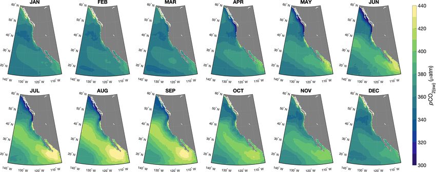
2084                                                               J. D. Sharp et al.: A monthly surface pCO2 product for the CCS

                                                                        2.3   Predictor variable acquisition and processing

                                                                        Of the 4 014 844 grid cells that represent the surface ocean
                                                                        gridded in three dimensions at 0.25◦ resolution over 276
                                                                        months (1998–2020) in the study region, just 1.25 % have
                                                                        an associated gridded pCO2(sw) value. To fill gaps in this
                                                                        dataset, relationships between pCO2(sw) and various predic-
                                                                        tor variables need to be determined. The predictor variables
                                                                        used in this study are primarily derived from satellite obser-
                                                                        vations or reanalysis models due to the condition that they
                                                                        be resolved with temporal and spatial continuity across the
                                                                        study region and selected time span.
                                                                           Predictor variables are intended to capture conditions that
                                                                        mechanistically influence pCO2(sw) (e.g., SST and atmo-
                                                                        spheric pCO2 ), serve as a proxy for mechanisms that influ-
                                                                        ence pCO2(sw) (e.g., sea surface chlorophyll), or, in the case
                                                                        of temporal and spatial information, constrain additional pat-
                                                                        terned variability not captured by the mechanistic variables
                                                                        alone. The chosen predictor variables for this study (Table 1)
                                                                        have all been used before for pCO2(sw) gap-filling methods
                                                                        (e.g., Landschützer et al., 2014; Gregor et al., 2018; Denvil-
                                                                        Sommer et al., 2019; Watson et al., 2020); temporal and spa-
                                                                        tial predictors were included to ensure robust representation
                                                                        of pCO2(sw) seasonal cycles (Gregor et al., 2017). Included
Figure 1. Annual mean pCO2(sw) from the 0.25◦ resolution grid-          in Table 1 are the sources of each dataset, the original resolu-
ded dataset computed as an average over the monthly climatology         tions of each dataset, and the steps that were taken to process
from 1998 to 2020 for each grid cell. The two extremes of the color     each dataset. Appendix A provides more detail about the ac-
bar can represent pCO2(sw) values less than or greater than the color   quisition and processing of the driver variables and includes
bar limits; the chosen range represents most of the values and em-      figures showing annual means of selected variables.
phasizes regional contrast.

                                                                        2.4   Construction of nonlinear relationships using
biases toward high-resolution measurement systems (Sabine                     random forest regression
et al., 2013).
   This bin-averaging procedure is identical to the one fol-            We used the random forest regression approach (Breiman,
lowed by the SOCAT team for producing monthly datasets                  2001) to identify relationships between pCO2(sw) and pre-
for coastal regions with 0.25◦ resolution as well as for open-          dictor variables in order to fill gaps in the gridded pCO2(sw)
ocean regions with 1◦ resolution (Sabine et al., 2013; Bakker           dataset. This method averages the results from a number
et al., 2016). However, here we produced a monthly grid-                of decision and/or regression trees (i.e., a “forest”) built
ded dataset with 0.25◦ resolution for a region of the north-            on bootstrapped replicates of the dataset – which individ-
eastern Pacific (15 to 60◦ N, 105 to 140◦ W) that spans both            ually have low bias and high variance – to produce a fi-
the coastal and open ocean. Means of pCO2(sw) from this                 nal regression model with reduced variance (Hastie et al.,
gridded dataset (averages over the monthly climatology from             2009). RFR is the machine-learning method of choice for
1998 to 2020 for each spatial grid cell) are shown in Fig. 1.           this study as early testing showed better performance than
Some of the apparent fine-scale spatial variability in this bin-        the SOM-FNN method in the northeastern Pacific. Further,
averaged map is not indicative of true environmental condi-             RFR is less computationally expensive than fitting a neural
tions but originates from the combination of large temporal             network and has been shown to produce results comparable
variability within each grid cell and uneven sampling of each           to the SOM-FFN approach in terms of overall performance
grid cell across and within years. This form of temporal vari-          (Gregor et al., 2017). It should be noted, however, that the
ability is exactly the kind of spurious result that advanced            two approaches differ mechanistically and therefore adapt
pCO2(sw) mapping techniques are intended to circumvent.                 to variability within a training dataset in different ways. Fi-
Figure B1 shows the number of years containing an observa-              nally, while RFR has been explored more frequently in recent
tion within each month of our gridded pCO2(sw) dataset. Un-             years as a method of spatiotemporal pCO2(sw) gap-filling
surprisingly, temporal coverage is highest close to the coast,          both globally (Gregor et al., 2017, 2018) and regionally in
especially in the summer months.                                        the Gulf of Mexico (Chen et al., 2019), far fewer RFR-based
                                                                        pCO2(sw) products exist than neural-network-based prod-

Earth Syst. Sci. Data, 14, 2081–2108, 2022                                              https://doi.org/10.5194/essd-14-2081-2022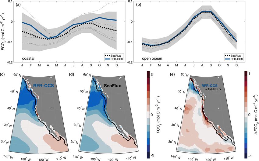
J. D. Sharp et al.: A monthly surface pCO2 product for the CCS                                                                              2085

Table 1. Sources of data for interpolation of surface pCO2 . Chlorophyll a (Chl) and mixed layer depth (MLD) were log10 -transformed to
produce a distribution of values that was closer to normal before constructing the regression model. Gaps in CHL data were filled by linear
interpolation over time within each grid cell (see Appendix A). Month of the year was transformed by cosine and sine functions to retain its
cyclical nature.

                                                                                          Original resolution
  Predictor variable              Source                  Citation                                                  Processing
                                                                                      Spatial            Temporal
  Sea surface temperature (SST)   OISSTv2                 Huang et al. (2021)         0.25◦              daily      monthly averages
  Sea surface salinity (SSS)      ECCO2                   Menemenlis et al. (2008)    0.25◦              daily      monthly averages
  Chlorophyll a (Chl;             SeaWiFS                 NASA Ocean Color            1/6◦               monthly    interpolated to 0.25◦
  log10 -transformed)             (1998–2002);                                                                      resolution
                                  MODIS (2003–2020)
  Wind speed (U )                 ERA5                    Hersbach et al. (2020)      0.25◦              monthly    none
  Atmospheric pCO2                NOAA marine             Dlugokencky et al. (2020)   sin(lat) of 0.05   weekly     monthly averages,
  (pCO2(atm) )                    boundary layer                                                                    interpolated to 0.25◦ lat.
                                  reference xCO2                                                                    resolution, multiplied by
                                                                                                                    NCEP sea level pressure
  Mixed layer depth (MLD;         HYCOM                   Chassignet et al. (2007)    1/6◦               monthly    interpolated to 0.25◦
  log10 -transformed)                                                                                               resolution
  Distance from shore             Calculated from         Greene et al. (2019)        –                  –          –
                                  gridded lat–long
  Year                            –                       –                           –                  –          –
  Month of year (converted to     –                       –                           –                  –          –
  two separate predictors using
  sine and cosine)

ucts. So, this study provides a good opportunity to further              into progressively smaller sets of similar observations un-
demonstrate the utility of RFR for producing monthly fields              til either the variance among the pCO2(sw) observations in
of pCO2(sw) , in this case on a regional scale in the northeast-         a node drops below a prescribed tolerance level or the num-
ern Pacific.                                                             ber of observations in the node reaches the user-defined min-
   Each decision tree within a random forest regression                  imum (MinLeafSize in Table 2). To ensure that the algorithm
model is built on a different subset of the training dataset             does not always pick the same predictor variable (e.g., the
(that contains both the predictor variables and corresponding            one most highly correlated with pCO2(sw) overall) for the
gridded pCO2(sw) values). This subset is generated by boot-              split at every node, we limit it to choosing from a different
strapping, in which a random set of training data points is se-          random subset of the predictor variables (equal in number
lected with replacement – meaning the same data point can                to NumPredictorsToSample in Table 2) at each node. This
be selected more than once (Breiman, 1996). The number of                introduces another “random” element into the tree-building
data points in the bootstrapped dataset is equal to a defined            process. The random forest contains a large number of these
fraction (InBagFraction in Table 2) of the original dataset;             regression trees (NumTrees in Table 2) each built on a dif-
however, a fraction equal to 1 does not mean the bootstrapped            ferent, random bootstrapped subsample of the training data.
dataset is identical to the original dataset because selection is        Once the random forest is built, a set of predictor vari-
made with replacement. Since each regression tree is built on            ables can be provided to the model and the average of the
a different subset of the training data, it will contain some-           pCO2(sw) values provided by each regression tree is used as
what different relationships between the predictor variables             the pCO2(sw) prediction for that particular set of inputs.
and the corresponding gridded pCO2(sw) values.                              We constructed an RFR model using the MATLAB Tree-
   The process of building a decision tree begins at the top             Bagger function with the predictor variables given in Ta-
“node” of the tree with the values of a single predictor vari-           ble 1 and the parameters given in Table 2, along with
able being used to split that tree’s bootstrapped subset of the          gridded pCO2(sw) values that were obtained as described
training dataset into two smaller subsets (not necessarily of            in Sect. 2.1 and 2.2. To produce the northeastern Pa-
equal size) containing the most similar pCO2(sw) observa-                cific random forest regressionpCO2(sw) product (RFR-CCS)
tions (i.e., sets of pCO2(sw) observations with the smallest             that is the main result of this work (Sharp et al., 2022;
variance among them). These subsets are then further divided             https://doi.org/10.5281/zenodo.5523389), the full dataset of

https://doi.org/10.5194/essd-14-2081-2022                                                 Earth Syst. Sci. Data, 14, 2081–2108, 2022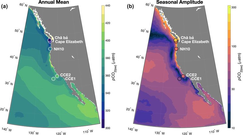
2086                                                            J. D. Sharp et al.: A monthly surface pCO2 product for the CCS

Table 2. Model parameters for the random forest regression. Parameter names are the default property names for the MATLAB TreeBagger
class.

   Parameter                  Explanation                                                                                        Value
   NumTrees                   Number of decision trees to build for random forest                                                1200
   MinLeafSize                Minimum number of observations in a given terminal node (i.e., the last node in a decision tree)      5
   NumPredictorsToSample      Number of randomly selected predictor variables to choose from at each node split                     6
   InBagFraction              Fraction of input data to sample with replacement for each bootstrapped dataset                     1.0

gridded pCO2(sw) values was used. For optimization and                dataset that was withheld from both the model training and
evaluation, subsets of the full dataset were used as described        model validation (i.e., the “test data”) was used to quantify
in the following sections.                                            the mapping uncertainties from the RFR approach (discussed
                                                                      further in Sects. 2.7 and 3.5). The predictor variable feature
2.5      Optimization of random forest regression model               importances for the final RFR-CCS fit are given in Fig. B2.

The predictor variables used (Table 1) and the values for the
                                                                      2.6    Evaluation of random forest regression approach
model parameters (Table 2) were determined by iteratively
                                                                             and resulting data product
optimizing the model performance. First, default model pa-
rameters were used to train an RFR model using a subset               Once predictor variables and model parameters were opti-
of the data for training (80 % of full dataset, distributed ran-      mized, the skill of the RFR approach was further evaluated
domly across the space and time domains of interest) and a            by splitting the full dataset into different subsets of train-
number of possible predictor variables: latitude, longitude,          ing data and test data. Evaluation models (RFR-CCS-Evals)
sea surface height, bottom depth, and those given in Table 1.         were constructed in three different ways: (1) by removing a
During model selection, the generalization skill for the RFR          random (20 %) subset of cruises and/or measurement plat-
model was assessed using a validation dataset comprised               forms from the training data (repeated 10 times with dif-
of 10 % of the full dataset, none of which was included in            ferent subsets removed each time; n = 10), (2) by removing
the training data. After the initial model fit, predictors with       all observations from every fifth year from the training data
a “feature importance” (computed during the RFR fit) sig-             (repeated five times such that data from every year was re-
nificantly lower than all other predictors were sequentially          moved from one of the trials; n = 5), and (3) by removing
dropped (latitude, longitude, and sea surface height), and            all moored autonomous pCO2(sw) measurements (i.e., dis-
this did not substantially change the training or validation          crete time series sites primarily located in the coastal ocean)
root mean squared error (RMSE). Remaining predictor vari-             from the training data (n = 1). The first two strategies were
ables were dropped one at a time for subsequent fits, and the         relevant for assessing bulk error statistics for the method ap-
goodness-of-fit and generalization skill of the model were as-        plied across the region and the third strategy for evaluating
sessed using the RMSE values calculated from applying the             the ability of the RFR to represent local seasonal variability
model to the training and validation datasets, respectively.          without the use of high-temporal-resolution mooring data.
The set of predictors with the lowest RMSE after dropping             These RFR-CCS-Evals are distinct model variants that are
one predictor was carried into the next iteration. If remov-          only used for assessment; the final RFR-CCS model uses all
ing a predictor did not increase the validation RMSE sig-             available training data.
nificantly, then that predictor was removed from the set of              Each data split for an RFR-CCS-Eval was applied di-
predictors (only bottom depth was dropped in this step). The          rectly to SOCATv2021 observations, before bin-averaging
final set of predictor variables is shown in Table 1.                 the data according to the procedure given in Sect. 2.2; as a
   Next, different values for model parameters (Table 2) were         result, a gridded training dataset and a gridded test dataset
tried iteratively with the retained predictors to identify the        were produced from each split. Data splits were performed
optimal values, again by minimizing the RMSE of the vali-             in this way to ensure that autocorrelation among measure-
dation dataset. Although lower values for the minimum ter-            ments from a specific platform did not bias the error statis-
minal node size performed better in this analysis, additional         tics. Each split was repeated n times, and error statistics (bias,
testing indicated that retaining the default value of 5 was           RMSE, and R 2 ) from comparing pCO2(sw) predicted from
important to prevent overfitting. To determine the appropri-          the RFR-CCS-Eval models versus pCO2(sw) from the grid-
ate number of trees, we examined how the out-of-bag mean              ded test dataset were averaged.
squared error changed as more and more trees were included               The final RFR-CCS data product was evaluated through
in the random forest (up to 5000 trees) and selected a num-           comparisons with gridded pCO2(sw) observations from SO-
ber of trees well past the point at which this error had sta-         CATv4 (Bakker et al., 2016) and pCO2(sw) observations from
bilized (1200 trees). Finally, the remaining 10 % of the full         surface ocean moorings (Sutton et al., 2019). Of the sur-

Earth Syst. Sci. Data, 14, 2081–2108, 2022                                              https://doi.org/10.5194/essd-14-2081-2022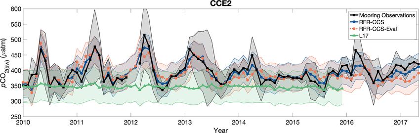
J. D. Sharp et al.: A monthly surface pCO2 product for the CCS                                                               2087

face ocean moorings within the study site that are not lo-         2.8    Calculation of CO2 flux
cated within an inland sea and have available data from all
                                                                   The flux of CO2 across the ocean–atmosphere interface
12 months of the year, four (CCE2, NH10, Cape Elizabeth,
                                                                   (FCO2 ) was calculated using a bulk formula:
Châ bá) are located within 40 km of shore and one (CCE1)
is about 215 km from shore. RFR-CCS was also compared to           FCO2 = kw × K0 × 1pCO2 ,                                    (3)
global-scale gap-filled pCO2(sw) products that are available
                                                                   where kw is the gas transfer velocity, K0 is the CO2
in the region. Namely, we focused on the coastal multi-month
                                                                   solubility constant, and 1pCO2 is the difference be-
pCO2(sw) product from Laruelle et al. (2017; i.e., L17) and
                                                                   tween CO2 partial pressure in seawater and in the overly-
the combined coastal and open-ocean pCO2(sw) climatology
                                                                   ing atmosphere (pCO2(sw) − pCO2(atm) ) The salinity- and
from Landschützer et al. (2020b; i.e., L20).
                                                                   temperature-dependent equations of Weiss (1974) were used
                                                                   to calculate K0 .
2.7   Uncertainty analysis                                            Gas transfer velocities were parameterized using a
Uncertainty in pCO2(sw) for each grid cell was calculated ac-      quadratic dependence on wind speed (Wanninkhof, 1992):
                                                                                     √
cording to the approach used by Landschützer et al. (2014,         kw = 0660 · U 2 · 660/Sc,                             (4)
2018) and Roobaert et al. (2019), in which total uncertainty
                                                                   where 0660 is a gas exchange coefficient normalized to Sc
in pCO2(sw) results from a combination of observational un-
                                                                   = 660, U 2 is the squared wind speed, and Sc is the Schmidt
certainty, mapping uncertainty, and gridding uncertainty. Ob-
                                                                   number for CO2 . Our calculations used 0660 = 0.276, which
servational uncertainty (θobs ) is uncertainty inherent to the
                                                                   is a gas exchange coefficient that is specific to ERA5 re-
original measurements of pCO2(sw) evaluated as the average
                                                                   analysis winds and scaled to a bomb-14 C flux estimate of
of reported uncertainties in the fCO2 (sw) observations from
                                                                   16.5 cm h−1 (Fay et al., 2021). Sc was calculated using the
our training dataset, which are flagged by SOCAT with a
                                                                   fourth-order polynomial fit of Wanninkhof (2014). U was
dataset QC flag of A or B (fCO2 (sw) accuracy of 2 µatm or
                                                                   obtained from ERA5 reanalysis (Hersbach et al., 2020). Flux
better) and of C or D (fCO2 (sw) accuracy of 5 µatm or bet-
                                                                   calculations used monthly averages of squared 3-hourly wind
ter); we weighted θobs by the number of observations as-
                                                                   speeds to retain the influence of the quadratic wind term (Fay
signed each flag. Mapping uncertainty (θmap ) is uncertainty
                                                                   et al., 2021).
contributed by the RFR mapping procedure and was evalu-
ated as separate values for the coastal (< 400 km from shore)
and open ocean (> 400 km from shore) using the mean of             3     Results and discussion
the root mean squared errors for a subset of test data (10 %)
withheld from both the model training data (80 %) and model        3.1    Evaluation by comparison to withheld data
validation data (10 %) (see Sect. 2.5). Gridding uncertainty       As described in Sect. 2.6, training and test datasets were cre-
(θgrid ) is uncertainty attributable to aggregating observations   ated by splitting the full dataset prior to bin-averaging. Eval-
into monthly 0.25◦ resolution grid cells and was evaluated         uation models (RFR-CCS-Evals) were constructed by fitting
as separate values for the coastal and open ocean by taking        RFR models using the various gridded training datasets. Val-
the average unweighted standard deviation among pCO2(sw)           ues of pCO2(sw) predicted by RFR-CCS-Evals were com-
values within each grid cell in which two or more platforms        pared to corresponding values from gridded test datasets. Er-
were represented. Grid cells with mooring observations were        ror statistics (bias, RMSE, and R 2 ) averaged over the n sets
excluded from the θgrid calculation to avoid the high num-         of evaluation tests are given in Table 3. When RFR-CCS is
ber of observations swamping the signal from other plat-           compared against all the gridded observations used to con-
forms. These three components were combined to obtain to-          struct it, error statistics are predictably strong (last row in
tal pCO2(sw) uncertainty (θpCO2 ) applicable to each open-         Table 3), with a mean bias of 0.00 µatm and an RMSE of
ocean grid cell and to each coastal grid cell:                     13.33 µatm (R 2 = 0.93). These error statistics demonstrate
            q                                                      the ability of the RFR model to fit the training data; the eval-
θpCO2 = θobs   2 + θ2 + θ2 .                                 (2)
                      map     grid                                 uation tests provide insight into the model’s ability to predict
                                                                   independent data.
Whereas θpCO2 represents the uncertainty in pCO2(sw) for a            Tests 1 and 2 are good indicators of the overall skill of
given grid cell in a given month, uncertainty averaged re-         RFR-CCS. The mean absolute bias for each of those tests is
gionally or over time will not scale exactly with θpCO2 due        less than 2 µatm, and the RMSEs are near or below 30 µatm.
to the spatial correlation of pCO2(sw) values and the autocor-     These error statistics can be compared with those of L17,
relation features of the model error (e.g., Landschützer et al.,   who obtained biases with a mean of 0.0 and RMSEs ranging
2014).                                                             from 20.5 to 53.1 µatm (mean of 39.2 µatm) for independent
                                                                   evaluations of coastal pCO2(sw) values fit using the SOM-
                                                                   FFN method in 10 separate global subregions at 0.25◦ res-
                                                                   olution. For an open-ocean comparison, Denvil-Sommer et

https://doi.org/10.5194/essd-14-2081-2022                                         Earth Syst. Sci. Data, 14, 2081–2108, 2022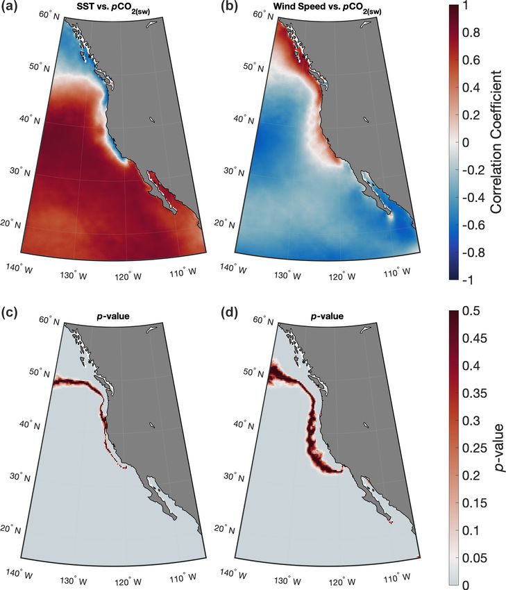
2088                                                                           J. D. Sharp et al.: A monthly surface pCO2 product for the CCS

Table 3. Error statistics for comparisons of predicted pCO2(sw) from evaluation models versus gridded pCO2(sw) from test datasets. The
number of times each test was repeated is given by n; where n is greater than 1, different subsets of data were removed for each iteration of
the test and error statistics are the mean of all iterations.

                                                Removed from                                       Mean bias         RMSE
                              Test no.                                                                                                 R2
                                                training dataset                                     (µatm)          (µatm)
                              1 (n = 10)        Random (20 %) subset of cruises                         −0.37         26.96         0.66
                              2 (n = 5)         Every fifth year                                         1.57         30.03         0.63
                              3 (n = 1)         Moored autonomous observations                           8.39         43.28         0.55
                              RFR-CCS           None; full dataset used                                 0.00∗        13.33∗        0.93∗
                            ∗ These statistics represent model training statistics (i.e., evaluated with the same data used to train the
                            model) rather than model validation statistics.

al. (2019) obtained an RMSE of 15.86 for an independent                                 at CCE2 with a mean bias of −44.2 µatm and an RMSE of
evaluation of pCO2(sw) values fit using a similar neural net-                           57.3 µatm (R 2 = 0.06). Notably, the mooring-excluded RFR-
work approach (LSCE-FFNN) for the subtropical North Pa-                                 CCS-Eval captures pCO2(sw) variability at CCE2 more ef-
cific (18 to 49◦ N) at 1◦ resolution. The error statistics for                          fectively than the L17 product, even though RFR-CCS-Eval
our study region, which spans the coastal to open-ocean con-                            was trained without mooring observations and the L17 train-
tinuum on a finely resolved spatial grid, lie comfortably be-                           ing dataset (i.e., SOCATv4) includes CCE2 mooring obser-
tween those coastal and open-ocean comparison points.                                   vations through 2014. Similar results are obtained for com-
   Test 3 is a good indicator of how well the RFR approach                              parisons to other mooring records (Table B1; Fig. B3), with
is able to reproduce the values and seasonalities of coastal                            RFR-CCS always producing the best error statistics (as ex-
pCO2(sw) at fixed locations when mooring data at a given lo-                            pected) and RFR-CCS-Eval always producing a better R 2
cation are not provided as training data, as each of the moor-                          than L17, indicating that coastal seasonality at mooring loca-
ings makes continuous pCO2(sw) measurements throughout                                  tions is better captured by our regional random forest regres-
the year and all but one of the mooring locations included                              sion model, even when mooring observations themselves are
in SOCATv2021 in this region are within 40 km of shore.                                 not included in the model training. This is an important con-
The positive mean bias (8.39 µatm) suggests that RFR-CCS                                clusion, especially in light of the recommendation by Hauck
somewhat overestimates pCO2(sw) at grid cells correspond-                               et al. (2020) that the inclusion of coastal areas and marginal
ing to mooring locations, but this is strongly influenced by                            seas in pCO2(sw) mapping methods will be critical for im-
high biases at the Cape Elizabeth and Châ bá mooring loca-                              proving the ocean carbon sink estimate. If these areas are to
tions (Table B1). The relatively high RMSE (43.28 µatm) is                              be included, it is sensible to attempt to capture their unique
a result of higher variability in coastal grid cells compared                           modes of variability as accurately as possible.
to the open ocean; this is confirmed by a comparison to the
offshore CCE1 mooring (Table B1), where the RMSE from
the mooring-excluded RFR-CCS-Eval is just 10.5 µatm.                                    3.2      Evaluation by comparison to global pCO2(sw)
   Figure 2 provides an example of one coastal mooring                                           products
record (CCE2, which is positioned on the shelf break off the                            Across the study area, values of pCO2(sw) from RFR-CCS
coast of Point Conception, CA, at 34.324◦ N, 120.814◦ W)                                were compared against corresponding values from L17 and
compared to pCO2(sw) predicted in the corresponding grid                                L20. For temporal compatibility with L17 and L20, a cli-
cell (centered at 34.375◦ N, 120.875◦ W) by the mooring-                                matology of average monthly values from RFR-CCS span-
excluded RFR-CCS-Eval model (Test 3) as well as the full                                ning 1998 to 2015 (RFR-CCS-clim) was created for these
RFR-CCS model. For comparison, pCO2(sw) in the same grid                                comparisons. Figure 3 shows mapped differences in annual
cell provided by the L17 coastal product is also shown. At                              means and seasonal amplitudes (calculated as the maximum
the CCE2 mooring location, RFR-CCS reproduces mooring-                                  climatological pCO2(sw) minus the minimum) of pCO2(sw)
observed monthly pCO2(sw) with a mean bias of −2.2 µatm                                 between RFR-CCS-clim versus L20 (top panels) and RFR-
and an RMSE of 16.1 µatm (R 2 = 0.81). These error statis-                              CCS-clim versus a climatological average of L17 (bottom
tics are expected to be relatively favorable, as the RFR-CCS                            panels); monthly mean differences in are given in Fig. B4.
model is trained using mooring observations from CCE2. In                                  The most notable feature of the annual mean difference
contrast, the mooring-excluded RFR-CCS-Eval reproduces                                  maps is that RFR-CCS-clim produces much higher annual
monthly mooring-observed pCO2(sw) at CCE2 with a mean                                   mean pCO2(sw) than both L17 and L20 in the nearshore
bias of −4.6 µatm and an RMSE of 28.9 µatm (R 2 = 0.41).                                coastal ocean and slightly higher pCO2(sw) in the remain-
This can be compared to the L17 coastal pCO2(sw) prod-                                  der of the study area. Similarly, RFR-CCS-clim produces
uct, which reproduces monthly mooring-observed pCO2(sw)                                 much higher seasonal variability than both L17 and L20 in

Earth Syst. Sci. Data, 14, 2081–2108, 2022                                                                     https://doi.org/10.5194/essd-14-2081-2022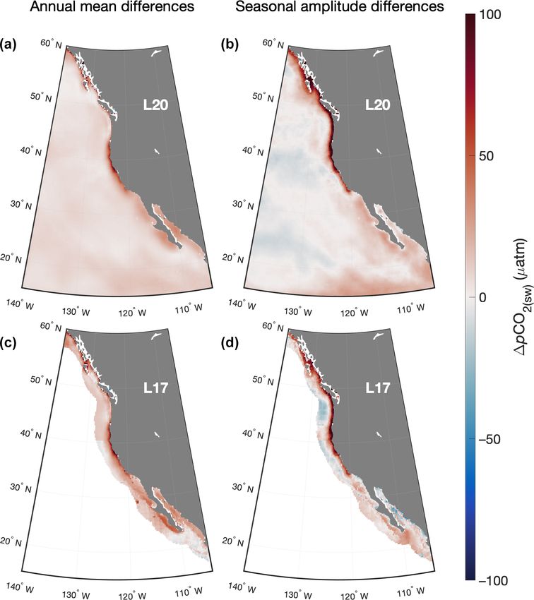
J. D. Sharp et al.: A monthly surface pCO2 product for the CCS 2089
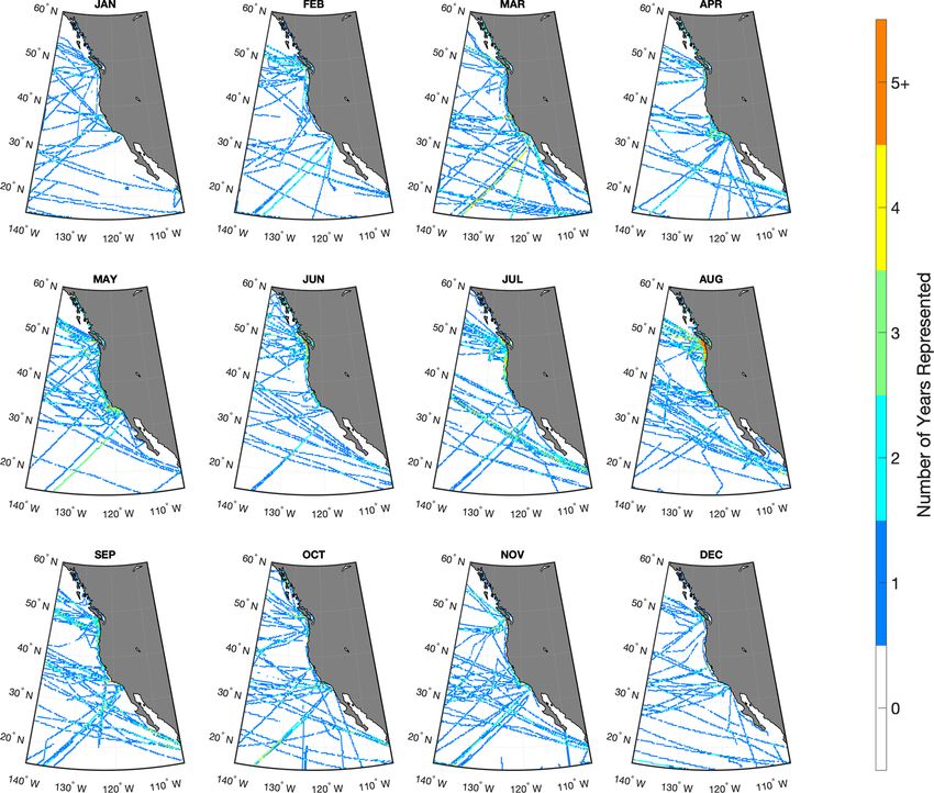
Figure 2. Monthly values of pCO2(sw) from mooring observations (black), RFR-CCS (blue), the mooring-excluded RFR-CCS-Eval model
(orange), and L17 (green). The envelope around the black line equals the standard deviation of all mooring observations within each month,
representing the natural variability of the 3-hourly mooring measurements; the envelopes around the blue and orange lines represent the
RFR-CCS and RFR-CCS-Eval results plus 1 standard uncertainty (43.6 µatm; Sect. 3.5); the envelope around the green line represents the
L17 data product plus the RMSE of an independent data evaluation in the province associated with CCE2 (52.5 µatm; Table 3 of Laruelle et
al., 2017; Province P7).
3.3 Evaluation by comparison to gridded observations
of pCO2(sw)
Values of pCO2(sw) from RFR-CCS, L17, and L20 were
compared against the SOCATv4 gridded pCO2(sw) data
product. SOCATv4 was used in the development of the
coastal L17 product, whereas SOCATv5 was used in the de-
velopment of the open-ocean product for the merged L20 cli-
matology, and SOCATv2021 was used in the development of
RFR-CCS. Therefore, comparisons were made to both the
gridded open-ocean observations (1◦ resolution) and gridded
coastal observations (0.25◦ resolution) from SOCATv4 to in-
clude only data points that were available to the training of
all three data products. To match the resolution of the gridded
open-ocean observations from SOCATv4, aggregation from
a 0.25◦ resolution grid to a 1◦ resolution grid was performed
for RFR-CCS, RFR-CCS-clim, and L20. L17 was only com-
pared to gridded coastal observations from SOCATv4 be-
cause the two are gridded to the same spatial resolution and
cover the same coastally limited spatial domain.
Figure 4 shows two-dimensional histograms of bin-
averaged differences between RFR-CCS-clim, L20, RFR-
CCS, and L17, each compared against gridded observations
Figure 3. Differences between annual means (a, c) and seasonal from SOCATv4. For comparisons to climatological products
amplitudes (b, d) of pCO2(sw) from RFR-CCS-clim versus the L20 (RFR-CCS-clim and L20), gridded SOCATv4 observations
climatology (a, b; RFR-CCS-clim – L20) and versus a climatologi- were averaged to a monthly climatology across 1998–2015
cal average of the L17 product (c, d; RFR-CCS-clim – L17).
for consistency with the products. The regional RFR-CCS
product and its climatology outperform both global SOM-
FFN products: RFR-CCS-clim shows better agreement with
the nearshore coastal ocean, especially north of about 34◦ N. gridded monthly means of observations from SOCATv4 than
On average, RFR-CCS-clim produces an area-weighted an- L20 (R 2 = 0.85 versus R 2 = 0.73), and RFR-CCS (within
nual mean pCO2(sw) that is greater than L17 by 19.0 µatm the coastally limited spatial domain of L17) shows better
and L20 by 8.4 µatm, as well as an area-weighted seasonal agreement with gridded observations from SOCATv4 than
amplitude that is greater than L17 by 13.0 µatm and L20 by L17 (R 2 = 0.96 versus R 2 = 0.61). In particular, the two
5.6 µatm. global products (L20 and L17) struggle to match pCO2(sw)
https://doi.org/10.5194/essd-14-2081-2022 Earth Syst. Sci. Data, 14, 2081–2108, 2022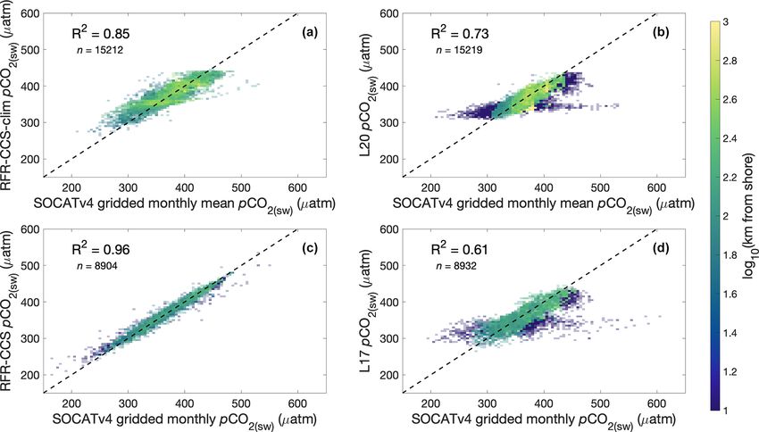
2090                                                           J. D. Sharp et al.: A monthly surface pCO2 product for the CCS

values in the nearshore coastal ocean (within 100 km of the         3.5   Uncertainty calculations
coast), indicated by dark blue cells in Fig. 4.
   Mismatches between global pCO2(sw) products and obser-           Three components comprised the estimate of uncertainty for
vations in the nearshore coastal ocean are not unexpected, as       pCO2(sw) values from RFR-CCS: observational uncertainty
regional error statistics for reconstructed global pCO2(sw) are     (θobs ), mapping uncertainty (θmap ), and gridding uncertainty
typically larger than the global mean error statistics (Laruelle    (θgrid ). According to the procedure detailed in Sect. 2.7,
et al., 2017; Landschützer et al., 2020c), and it is generally      θobs was calculated as 3.3 µatm, θmap as 4.4 µatm for the
more challenging to model pCO2(sw) in environments with             open ocean and 35.3 µatm for the coastal ocean, and θgrid as
high temporal and spatial variability, such as in the nearshore     3.7 µatm for the open ocean (n = 268) and 25.1 µatm for the
coastal ocean (Landschützer et al., 2014). This result em-          coastal ocean (n = 889). These three components were com-
phasizes the importance of carefully addressing nearshore           bined to obtain total pCO2(sw) uncertainty (θpCO2 ) accord-
pCO2(sw) when constructing global products if one hopes to          ing to Eq. (2), resulting in θpCO2 equal to 6.6 µatm for the
achieve an accurate representation of coastal ocean variabil-       open ocean and 43.4 µatm for the coastal ocean. The open-
ity. This may be achieved (1) by using a greater number of          ocean value determined through this analysis compares well
model clusters for coastal ocean reconstructions (L17 uses          with the grid-level uncertainty estimated in open-ocean grid
just 10 biogeochemical clusters for the global coastal ocean),      cells by Landschützer et al. (2014), which ranged from 8.6 to
(2) by increasing the spatial and/or temporal resolution of         17.7 µatm for different regions. The large coastal uncertainty
pCO2(sw) data products to better account for small-scale vari-      value emphasizes the high degree of variability in monthly
ability (Gregor et al., 2019), (3) by carefully accounting for      pCO2(sw) near ocean margins.
mismatches between the temperature (and salinity) at which             As noted in Sect. 2.7, uncertainties reported here are ap-
pCO2(sw) is measured versus that at which it is reported in         propriate for a given grid cell (i.e., monthly 0.25◦ latitude
surface data products (Ho and Schanze, 2020; Watson et al.,         by 0.25◦ longitude bin). Values averaged over time or over
2020), or (4) by taking an ensemble approach to pCO2(sw)            larger regions will have reduced pCO2(sw) (and CO2 flux) un-
gap-filling to reduce errors overall, especially in undersam-       certainties due to the spatiotemporal correlation of pCO2(sw)
pled regions (Gregor et al., 2019; Fay et al., 2021). Ulti-         and the autocorrelation features of the model error (e.g.,
mately, it will be critical to continue to expand our observa-      Landschützer et al., 2014).
tional capabilities by means of shipboard underway systems
(Pierrot et al., 2009), uncrewed surface vehicles (Meinig et        3.6   Spatial and seasonal patterns of sea surface pCO2
al., 2015; Sutton et al., 2021), biogeochemical Argo floats
(Roemmich et al., 2019), moored buoys (Sutton et al., 2019),        In the open ocean, relatively high pCO2(sw) values can be
and other platforms, as well as to make strides toward incor-       observed off southern Baja California (Fig. 6a) and extend-
porating these novel measurements into pCO2(sw) gap-filling         ing toward the northwest, especially during summer months
schemes (Gregor et al., 2019; Djeutchouang et al., 2022).           and into autumn (Fig. 7) when higher sea surface tempera-
                                                                    tures drive higher pCO2(sw) (Nakaoka et al., 2013). This area
3.4    Evaluation by comparison to seasonal observations            also corresponds to low chlorophyll (Fig. A2) and the low-
       of pCO2(sw) at ocean moorings                                est wind speeds across the study region (Fig. A4), suggesting
                                                                    that a lack of nutrient delivery from deep convection may be
Values of pCO2(sw) from RFR-CCS-clim, L17, and L20 were             limiting biological production, also driving high pCO2(sw) .
compared against monthly climatologies from mooring ob-             Relatively low open-ocean pCO2(sw) values can be observed
servations to evaluate how well each product captured sea-          in the northern part of the study region from about 45 to
sonal variability at fixed time series sites. Figure 5 shows        60◦ N (Fig. 6a). Wintertime cooling drives low pCO2(sw) in
climatologies of mooring-observed pCO2(sw) (each averaged           this area, though that effect is compensated for by dissolved
over available years and normalized to their annual mean)           inorganic carbon (DIC) brought to the surface by deep win-
compared to pCO2(sw) from RFR-CCS-clim, L20, and clima-             ter mixing (Ishii et al., 2014). Figure B5 illustrates competing
tological monthly averages of L17 (each normalized to their         effects between temperature and winds by displaying corre-
annual mean) in the grid cell corresponding to the mooring          lations between SST and pCO2(sw) , which are mainly pos-
location. Overall, RFR-CCS-clim does a much better job of           itive below 50◦ N, and between wind speed and pCO2(sw) ,
capturing the variability in mooring observations than either       which are mainly positive above 50◦ N.
L17 or L20 (Table 4).                                                  In the summer, high biological production in the northern
                                                                    portion of the study region (Fig. A2) removes DIC, keep-
                                                                    ing pCO2(sw) relatively low. This low-pCO2(sw) region ex-
                                                                    tends southward along the California coast to about 34◦ N
                                                                    between both offshore and nearshore high-pCO2(sw) waters.
                                                                    The southward extension of the low-pCO2(sw) region is con-
                                                                    sistent with what we know about the dynamics of the CCS:

Earth Syst. Sci. Data, 14, 2081–2108, 2022                                          https://doi.org/10.5194/essd-14-2081-2022
J. D. Sharp et al.: A monthly surface pCO2 product for the CCS 2091
Figure 4. Two-dimensional histograms showing bin-averaged comparisons of pCO2(sw) from (a) RFR-CCS-clim and (b) L20 to SOCATv4
gridded observations that have been averaged to a climatology, as well as comparisons of pCO2(sw) from (c) RFR-CCS and (d) L17 to
SOCATv4 gridded monthly observations in the coastally limited spatial domain of L17. Grid cells are color-coded by the average base-10
logarithm of distance from shore (km) of the observations included within each bin; the transparency of each grid cell is set by the relative
number of observations within each bin.
Table 4. Seasonal amplitudes of pCO2(sw) (µatm) from mooring observations and corresponding grid cells of climatological averages (from
1998–2015) of RFR-CCS-clim, L17, and L20.
Mooring CCE1 CCE2 Cape Elizabeth Châ bá NH10
Mooring 36.3 76.5 116.7 163.0 94.5
RFR-CCS-clim 32.4 64.0 133.6 129.5 97.4
L17 21.1 6.3 37.2 35.6 26.9
L20 23.0 6.3 22.1 21.2 18.9
a narrow band of nearshore waters is high in DIC in the (Fiechter et al., 2014; Turi et al., 2014; Deutsch et al., 2021)
spring and summer due to the direct effects of wind-driven studies. It corresponds to naturally low surface pH values
upwelling (Fig. 7), but a wider band of waters farther off- and aragonite saturation states, which will be exacerbated
shore is lower in DIC due to drawdown by high biologi- by increasing atmospheric CO2 concentrations (Gruber et al.,
cal production stimulated by nutrients delivered to the eu- 2012; Hauri et al., 2013), with likely deleterious effects for
photic zone by upwelling (Hales et al., 2005; Fassbender et calcifying organisms (Feely et al., 2008).
al., 2011; Fiechter et al., 2014; Turi et al., 2014). Relatively low coastal pCO2(sw) values (340 µatm or
In the coastal ocean, high pCO2(sw) occurs in the central lower) develop during April off the coasts of Oregon, Wash-
CCS (∼ 34 to ∼ 42◦ N), with values of 400 µatm or greater ington, and Vancouver Island and propagate northward to-
beginning in April off Pt. Conception (34◦ N) and propagat- ward southern Alaska through September (Fig. 7). Low sum-
ing northward to around Cape Arago (43◦ N) through Oc- mertime pCO2(sw) in the northern CCS (∼ 42 to ∼ 50◦ N) has
tober (Fig. 7). This corresponds to the latitudinal band of been demonstrated before (Hales et al., 2005, 2012; Evans
the CCS with the strongest and most consistent equatorward et al., 2011; Fassbender et al., 2018) and corresponds to the
winds (Huyer, 1983), which induce upwelling of CO2 -rich weaker and more variable equatorward winds in summer in
subsurface waters by wind-driven Ekman transport very near the northern CCS (Checkley and Barth, 2009) as well as
the coast and wind-stress-curl-driven Ekman pumping far- the effect of DIC drawdown by high primary productivity,
ther offshore (Checkley and Barth, 2009). This nearshore which offsets upwelling-induced increases in pCO2(sw) . Pri-
band of high summertime pCO2(sw) has been previously re- mary productivity in the northern CCS can be enhanced rel-
ported by observational (Hales et al., 2012) and modeling ative to the rest of the CCS due to factors like riverine nu-
https://doi.org/10.5194/essd-14-2081-2022 Earth Syst. Sci. Data, 14, 2081–2108, 20222092 J. D. Sharp et al.: A monthly surface pCO2 product for the CCS Figure 5. Climatological mean pCO2(sw) from five NOAA ocean moorings and the corresponding grid cells in RFR-CCS-clim, L20, and a climatological average of L17. Shading represents the standard deviation of all monthly values for each mooring or data product. trient delivery and distribution, submarine canyon-enhanced region, pCO2(sw) is generally lower than in offshore waters upwelling, and physical retention of phytoplankton blooms of the same latitude, which matches previous results well (Hickey and Banas, 2008). (Fig. 6a; Hales et al., 2012; Deutsch et al., 2021). One ex- The coastal ocean from Vancouver Island northward is a ception is directly off the southern tip of Baja California, high-pCO2(sw) region from October to March (Fig. 7), which where especially high summertime pCO2(sw) is observed. is broadly consistent with observations of high pCO2(sw) in This may in part reflect the tendency for wind-driven up- the western Canadian coastal ocean during autumn and win- welling to bring significant amounts of CO2 -rich subsurface ter (Evans et al., 2012, 2022). This high pCO2(sw) is per- waters to the surface just south of major topographic features haps due to the influence of deep tidal mixing (Tortell et al., (Van Geen et al., 2000; Friederich et al., 2002; Fiechter et al., 2012) and wintertime light limitation of DIC drawdown by 2014). Coastal pCO2(sw) within the Gulf of California (GoC) primary production. The northern coastal area shifts to a low- appears to be strongly influenced by thermally induced sea- pCO2(sw) region from April to September, again consistent sonal effects, though the lack of observational data coverage with observations (Evans et al., 2012, 2022) and likely re- in the GoC within SOCATv2021 (Fig. 1), especially within flecting surface DIC drawdown by primary production in the the nonsummer months (Fig. B1), may mask more dynamic region (Ianson et al., 2003). variability. The coastal ocean from the Southern California Bight The seasonal amplitude of pCO2(sw) (Fig. 6b) exhibits in- (SCB) southward along Baja California (∼ 22 to ∼ 34◦ N) teresting variation in the central and northern CCS. Here, shows relatively low pCO2(sw) seasonality (Fig. 6b). In this nearshore seasonality is extremely high due to dominant ef- Earth Syst. Sci. Data, 14, 2081–2108, 2022 https://doi.org/10.5194/essd-14-2081-2022
J. D. Sharp et al.: A monthly surface pCO2 product for the CCS                                                               2093

Figure 6. Annual mean pCO2(sw) (a) and the seasonal amplitude of pCO2(sw) (b) from RFR-CCS. Also shown are annual mean pCO2(sw)
and the seasonal amplitude of pCO2(sw) measured at ocean mooring locations.

Figure 7. Monthly mean pCO2(sw) fields from RFR-CCS.

fects from upwelling and primary production; however, sea-           3.7      Carbon uptake in the RFR-CCS domain
sonality farther offshore is extremely low, likely due to com-
pensating effects by thermally driven changes to pCO2(sw)
(high temperature in summer increases pCO2(sw) , low tem-            A recently published data product (SeaFlux; Gregor and Fay,
perature in winter decreases pCO2(sw) ) and biologically or          2021) described by Fay et al. (2021) harmonizes calculations
physically driven changes to pCO2(sw) (high primary produc-          of global CO2 flux by standardizing the areas covered by dif-
tion in summer decreases pCO2(sw) , deep mixing in winter            ferent global pCO2(sw) products and by scaling the gas ex-
increases pCO2(sw) ). Elsewhere, a hotspot of high seasonal-         change coefficient to different wind products. As part of this
ity exists offshore around 40◦ N, possibly due to thermal con-       procedure, the L20 climatology is used to fill spatial gaps in
trol of pCO2(sw) without strong biophysical compensatory             some of the pCO2(sw) products. As we have demonstrated
effects.                                                             here, filling gaps with this climatology may result in an un-
                                                                     derestimate of the seasonal pCO2(sw) cycle in certain loca-
                                                                     tions, especially nearshore (Fig. 5). For comparison we cal-
                                                                     culate monthly CO2 flux in our study region from SeaFlux

https://doi.org/10.5194/essd-14-2081-2022                                            Earth Syst. Sci. Data, 14, 2081–2108, 2022
You can also read