A revised dry deposition scheme for land-atmosphere exchange of trace gases in ECHAM/MESSy v2.54
←
→
Page content transcription
If your browser does not render page correctly, please read the page content below

Geosci. Model Dev., 14, 495–519, 2021
https://doi.org/10.5194/gmd-14-495-2021
© Author(s) 2021. This work is distributed under
the Creative Commons Attribution 4.0 License.

A revised dry deposition scheme for land–atmosphere exchange
of trace gases in ECHAM/MESSy v2.54
Tamara Emmerichs1 , Astrid Kerkweg1 , Huug Ouwersloot2 , Silvano Fares3 , Ivan Mammarella4 , and
Domenico Taraborrelli1
1 Institute of Energy and Climate Research 8, Troposphere, Forschungszentrum Jülich, Jülich, Germany
2 Max   Planck Institute for Chemistry, Mainz, Germany
3 National Research Council, Institute of Bioeconomy, Rome, Italy
4 Institute for Atmospheric and Earth System Research/Physics, Faculty of Science, University of Helsinki, Helsinki, Finland

Correspondence: Domenico Taraborrelli (d.taraborrelli@fz-juelich.de)

Received: 14 May 2020 – Discussion started: 17 June 2020
Revised: 20 November 2020 – Accepted: 6 December 2020 – Published: 26 January 2021

Abstract. Dry deposition to vegetation is a major sink of         been revised accordingly. The comparison of the simulation
ground-level ozone and is responsible for about 20 % of the       results with measurement data at four sites shows that the
total tropospheric ozone loss. Its parameterization in atmo-      new scheme enables a more realistic representation of dry
spheric chemistry models represents a significant source of       deposition. However, the representation is strongly limited
uncertainty for the global tropospheric ozone budget and          by the local meteorology. In total, the changes increase the
might account for the mismatch with observations. The             dry deposition velocity of ozone up to a factor of 2 glob-
model used in this study, the Modular Earth Submodel Sys-         ally, whereby the highest impact arises from the inclusion of
tem version 2 (MESSy2) linked to the fifth-generation Euro-       cuticular uptake, especially over moist surfaces. This corre-
pean Centre Hamburg general circulation model (ECHAM5)            sponds to a 6 % increase of global annual dry deposition loss
as an atmospheric circulation model (EMAC), is no excep-          of ozone resulting globally in a slight decrease of ground-
tion. Like many global models, EMAC employs a “resis-             level ozone but a regional decrease of up to 25 %. The change
tance in series” scheme with the major surface deposition via     of ozone dry deposition is also reasoned by the altered loss
plant stomata which is hardly sensitive to meteorology, de-       of ozone precursors. Thus, the revision of the process param-
pending only on solar radiation. Unlike many global models,       eterization as documented here has, among others, the poten-
however, EMAC uses a simplified high resistance for non-          tial to significantly reduce the overestimation of tropospheric
stomatal deposition which makes this pathway negligible in        ozone in global models.
the model. However, several studies have shown this process
to be comparable in magnitude to the stomatal uptake, espe-
cially during the night over moist surfaces. Hence, we present
here a revised dry deposition in EMAC including meteoro-          1   Introduction
logical adjustment factors for stomatal closure and an explicit
cuticular pathway. These modifications for the three stomatal     Ground-level ozone is a secondary air pollutant which is
stress functions have been included in the newly developed        harmful for humans and ecosystems. Besides chemical de-
MESSy VERTEX submodel, i.e. a process model describ-              struction, a large fraction of it is removed by dry deposi-
ing the vertical exchange in the atmospheric boundary layer,      tion which accounts for about 20 % of the total O3 loss
which will be evaluated for the first time here. The scheme       (Young et al., 2018). The process description of dry deposi-
is limited by a small number of different surface types and       tion considers boundary-layer meteorology (e.g. turbulence),
generalized parameters. The MESSy submodel describing             chemical properties of the trace gases and surface types.
the dry deposition of trace gases and aerosols (DDEP) has         In most global models, dry deposition of trace gases is pa-
                                                                  rameterized using the “resistance in series” analogy by We-

Published by Copernicus Publications on behalf of the European Geosciences Union.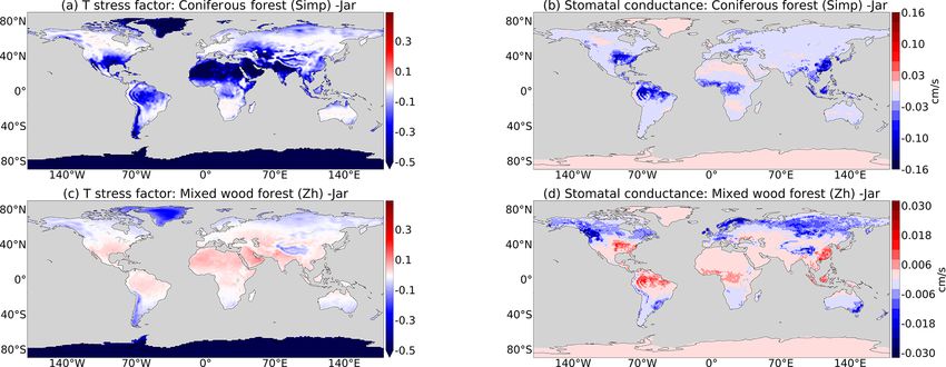
496                                                                                       T. Emmerichs et al.: Dry deposition

sely (1989). The largest deposition rates of ozone occur over      position at the leaf covering of plants. Zhang et al. (2002)
dense vegetation (Hardacre et al., 2015) where it mainly fol-      firstly derived a parameterization from field studies which es-
lows two pathways: through leaf openings (stomata) and to          tablishes the important link of this process to meteorology. In
leaf waxes (cuticle) (Fares et al., 2012). Thereby, stomatal       general, findings by Solberg et al. (2008), Andersson and En-
uptake is commonly parameterized following the empirical           gardt (2010) and Wong et al. (2019) highlight the importance
multiplicative approach by Jarvis (1976) which uses a pre-         of considering the dry deposition–meteorology dependence
defined minimum resistance and multiple environmental re-          in global models. Such an extension would realistically en-
sponse factors like in Zhang et al. (2003), Simpson et al.         hance the sensitivity of dry deposition to climate variability
(2012) and Emberson et al. (2000). More advanced formu-            and would result in a more accurate prediction of ground-
lations often used by land surface models (Ran et al., 2017;       level ozone.
Val Martin et al., 2014) are based on the CO2 assimilation            Given the importance of ozone as a major tropospheric
by plants during photosynthesis (Ball et al., 1987; Collatz        oxidant, air pollutant and greenhouse gas, an accurate rep-
et al., 1992). Both approaches rely on the choice and con-         resentation of dry deposition is desirable (Jacob and Win-
straints of ecosystem-dependent parameters and have differ-        ner, 2009). Additionally, the significance of a realistic repre-
ent advantages (Lu, 2018). A further role in coupling stom-        sentation of land–atmosphere feedbacks rises in light of the
ata to ecosystems is played by stomatal optimization models,       changing Earth’s climate with the projected increase of ex-
whereas optimal stomatal activity with a maximum amount            treme events’ frequency and intensity (Coumou and Rahm-
of carbon gain and a minimum loss of water is calculated           storf, 2012).
based on ecophysiological processes (e.g. Cowan and Far-              Here, we present a revision of the existing Wesely-based
quhar, 1977). Of particular interest are stomatal optimization     dry deposition scheme in the Modular Earth Submodel Sys-
models which, based on ecophysiological processes, maxi-           tem (MESSy), which has a very simplified representation
mize carbon gain while minimizing water loss. According            of vegetation and soil. The modifications are done by well-
to Wang et al. (2020), these models are promising in repre-        established findings about the controls of stomatal and cutic-
senting stomatal behaviour and improving carbon cycle mod-         ular uptake of trace gases. The calculation of stomatal depo-
elling. Non-stomatal deposition has been less investigated by      sition fluxes is extended by including the vegetation density,
now; therefore, most models use predefined constant resis-         two meteorological adjustment factors and an improved soil
tances or scale it with leaf area index (e.g. Val Martin et al.,   moisture availability function for plant stomata following the
2014; Simpson et al., 2012), while some apply an explicit          multiplicative algorithm by Jarvis (1976). For the first time
parameterization based on the observational findings of en-        in MESSy, a parameterization for cuticular dry deposition
hance cuticular uptake under leaf surface wetness (Altimir         dependent on important meteorological and environmental
et al., 2006).                                                     variables is implemented explicitly (Zhang et al., 2003). In
   The different parameterizations of the (surface) resistances    Sect. 2, a description of the model setup and the simulations
cause main model uncertainties in computing dry deposition         is provided, whereas especially the transition to the new ver-
fluxes of trace gases, which depend on the response to hy-         tical exchange scheme is described in detail. Subsequently,
droclimate and land-type-specific properties (Hardacre et al.,     the new VERTEX scheme is evaluated. In Sect. 4, the im-
2015; Wu et al., 2018; Wesely and Hicks, 2000). Thereby, it        pact of the changes on ozone dry deposition is evaluated
has been shown that the original Wesely-based parameteri-          on daily and seasonal scales by comparison with measure-
zation generally captures well the seasonal and diurnal cy-        ments at four different sites. Here, advantages, uncertainties
cles of dry deposition velocity, whereas model–observation         and missing processes in the revised scheme are identified.
discrepancy at seasonal scales arises from biased land type        Next, the global impact on ground-level ozone is assessed by
and leaf area index input data (Silva and Heald, 2018). Wong       separating the effect of the different implemented parameter-
et al. (2019) stated that discrepancies of up to 8 ppb in          izations. Then, Sect. 6 provides a description of the uncer-
ground-level ozone arise from different parameterizations.         tainties in modelling stomatal conductance and Sect. 7 com-
   The current dry deposition scheme of EMAC uses six sur-         prises an investigation of the sensitivity to model resolution.
face types, where the parameterized processes represent the        Section 8 summarizes the main findings and the remaining
forest canopy as a whole (big-leaf approach). Thereby, the         process and model uncertainties which form the basis for the
uptake over vegetation relies on stomatal deposition as the        provided recommendations. Section 9 describes planned fu-
only pathway determined by the photosynthetically active           ture developments.
radiation (Kerkweg et al., 2006). According to Fares et al.
(2012) and Rannik et al. (2012), the stomatal uptake in pa-
rameterizations often lacks the dependence on meteorolog-          2   Model description
ical and environmental variables (leaf area index, tempera-
ture, vapour pressure deficit). Moreover, several studies (e.g.    This study uses the ECHAM/MESSy atmospheric chemistry
Hogg et al., 2007; Fares et al., 2012; Clifton et al., 2017)       model. MESSy v2.54 (Jöckel et al., 2010) provides a flexible
found the contribution of an additional process to dry de-         infrastructure for coupling processes to build comprehensive

Geosci. Model Dev., 14, 495–519, 2021                                                https://doi.org/10.5194/gmd-14-495-2021

T. Emmerichs et al.: Dry deposition                                                                                          497

Earth system models (ESMs) and is utilized here with the
fifth-generation European Centre Hamburg general circula-
tion model (ECHAM5; Roeckner et al., 2003) as an atmo-
spheric general circulation model. The dry deposition pro-
cess of gases is calculated within the submodel DDEP (Kerk-
weg et al., 2006). This is described in Sect. 2.2. It relies on
the VERTEX vertical exchange submodel (Sect. 2.1), former
E5VDIFF, which contains the calculation of stomatal uptake
(Eq. 5) and soil moisture stress (Eq. 12). The stomatal up-
take parameterization is the base for the evapotranspiration
scheme in VERTEX (Appendix B) which also incorporates
the soil moisture stress.

2.1   The new VERTEX vertical exchange submodel

The VERTEX submodel represents land–atmosphere ex-
change and vertical diffusion as an alternative to the default
E5VDIFF submodel in ECHAM5/MESSy. In 2016, Huug
Ouwersloot branched VERTEX off from E5VDIFF. He opti-
mized the code and applied bug fixes. This includes changes
in calculation of the transfer coefficients for vertical diffu-   Figure 1. Dry deposition resistance analogy (adapted from Zhang
sion, the latent heat vaporization, the convective transfer co-   et al., 2003); modified resistors are marked with red boxes.
efficient, the storage of the friction velocity, the roughness
length over sea, the kinematic heat and moisture fluxes and
the 2 and 10 m friction velocity. A detailed description can      trace gas concentration C(X) (in molecules m−3 ):
be found in the Supplement.
                                                                  fd (X) = −vd (X) · C(X).                                   (2)
2.2   Dry deposition over vegetation                              The total resistance over land combines the resistances over
                                                                  snow, soil, vegetation (veg) and wet skin (ws) weighted by
Dry deposition of trace gases to vegetation is calculated ac-
                                                                  the respective land-covered fraction of a grid box (Kerkweg
cording to the multiple resistance scheme by Wesely (1989)
                                                                  et al., 2006). In the following, only the latter two are con-
shown in Fig. 1. The scheme, originally designed for a re-
                                                                  sidered. The resistances Ra and Rqbr are commonly param-
gional model with 11 land types and five seasonal cate-
                                                                  eterized with standard formulations from micrometeorology
gories, is used here with six generalized land types (Kerkweg
                                                                  (Kerkweg et al., 2006; Wesely and Hicks, 1977). For the sur-
et al., 2006). This was adapted by Ganzeveld and Lelieveld
                                                                  face resistance over vegetation (Rs,veg ), the parameterization
(1995) to the surface scheme of the ECHAM climate model
                                                                  according to Zhang et al. (2003) is used:
(Klimarechenzentrum et al., 1992). The vegetation canopy
is represented as one system; i.e. the detailed structure and         1               1
plant characteristics are neglected (one big-leaf approach).                 =
                                                                  Rs,veg (X) Rcan + Rs,soil (X)
Only one assumption about the canopy structure is made:
                                                                           1                   1
the leaves are horizontally oriented and the leaf density is        +           +                           ,                (3)
uniformly vertically distributed (Sellers, 1985). This is re-          Rcut (X)   Rstom,corr (X) + Rmes (X)
                                                                       |               {z                 }
quired in the formula for the calculation of stomatal resis-                       Rleaf (X)
tance (Eq. 5).
   The resistances (in s m−1 ) in the big-leaf approach account   which consists of the soil resistance (Rs,soil (X)), the in-
for mass and energy transfer mainly exerted by the bound-         canopy aerodynamic resistance (Rcan ) (as in Kerkweg et al.,
ary layer turbulence (Ra ), molecular diffusion via the quasi-    2006) and the leaf resistance (Rleaf (X)). The gas uptake by
laminar boundary layer (Rqbr ) and heterogeneous losses at        leaves (leaf) can be separated in two parallel pathways: the
the surface (Rs ) (Kerkweg et al., 2006). With these, the dry     cuticular (cut) and the stomatal (stom) with its associated
deposition velocity vd of a trace gas X (in s m−1 ) is defined    mesophilic pathway (mes), where the latter has negligible re-
as follows:                                                       sistance for ozone and highly soluble species (Wesely, 1989).
                      1                                           In contrast to the default formulation in MESSy (Eq. A1),
vd (X) =                            .                       (1)   the resistances in the updated scheme are provided at canopy
           Ra + Rqbr (X) + Rs (X)
                                                                  scale in order to avoid linear scaling with the leaf area in-
The dry deposition flux fd (X) (in molecules m−2 s−1 ) is de-     dex (LAI, area of leaves [m2 ]/surface area [m2 ]). In fact,
termined by multiplying the dry deposition velocity with the      the linear scaling of resistances with LAI assumes that the

https://doi.org/10.5194/gmd-14-495-2021                                               Geosci. Model Dev., 14, 495–519, 2021
498                                                                                                T. Emmerichs et al.: Dry deposition

leaves act in parallel and overestimates the uptake for high
LAI values (> 3–4) (Ganzeveld et al., 1998; Baldocchi et al.,
                                                                  Rstom (PAR, LAI) =
1987). Furthermore, the quasi-laminar boundary resistance
of individual leaves is included through the cuticular deposi-                                       kc
                                                                     h                                                           i ,    (5)
tion scheme (see Sect. 2.2.2), whereas Rqbr,veg is a separate              b             d exp(kLAI)+1               d+exp(−kLAI)
                                                                         dPAR   ln            d+1         − ln           d+1
term in the old formulation (Eq. A1).
   Due to the importance of stomatal and cuticular uptake for     where k = 0.9 is the extinction coefficient, c = 100 s m−1
ozone dry deposition, their respective parameterizations are      is the minimum stomatal resistance, and a = 5000 J m−3 ,
modified in this study (see Sect. 2.2.1 and 2.2.2). Also, ozone                            a+b·c
                                                                  b = 10 W m−2 and d = c·PAR     are fitting parameters (Sellers,
deposition to soil might be an important pathway (Schwede         1985). For historical reasons, LAI was set to 1 in order to
et al., 2011; Fares et al., 2012) but process understanding re-   obtain the stomatal resistance at leaf level (Ganzeveld and
mains limited due to scant observational constraints (Clifton     Lelieveld, 1995). This has been changed and the seasonal
et al., 2020b, a). Stella et al. (2011) showed an exponen-        evolution of stomatal resistance now follows the LAI which,
tial increase of soil resistance with surface relative humidity   in our study, is based on a 5-year climatology of monthly
in three agricultural data sets which, however, varies much       normalized difference vegetation index (NDVI) satellite data
between different sites (Stella et al., 2019) and contradicts     (Ganzeveld et al., 2002).
previous findings (Altimir et al., 2006; Lamaud et al., 2002;        First, the stomatal resistance is corrected by the inverse
Zhang et al., 2002). Models by, e.g. Mészáros et al. (2009);      of the temperature stress factor (1/f (T )) derived by Jarvis
Lamaud et al. (2009) apply a linear dependence on soil wa-        (1976):
ter content for parameterizing soil resistance. These parame-
terizations rely on input variables like the minimum soil re-     f (T ) = b3 (T − Tl )(Th − T )b4                                          (6)
sistance (Stella et al., 2011) which introduce an uncertainty                                       −b4
                                                                  b3 = (T0 − Tl )(Th − T0 )                                                 (7)
due to measurement constraints. Also, the performance of a
mechanistic model as proposed by Clifton et al. (2020b) de-       b4 = (Th − T0 )/(Th − Tl ),                                               (8)
pends on many input variables and parameters whose esti-
                                                                  where the empirical parameters are Th = 318.15 K, Tl =
mation is challenging and mostly biome dependent. Due to
                                                                  268.15 K and T0 = 298.15 K.
these uncertainties and limitations, the current parameteriza-
                                                                     Secondly, following the analysis by Katul et al. (2009),
tion of soil resistance in MESSy (see Kerkweg et al., 2006
                                                                  a stress factor dependent on vapour pressure deficit
for details) was not modified in this study.
                                                                  (1/f (VPD)) was added to the calculation of stomatal resis-
2.2.1   Uptake through plant stomata                              tance in VERTEX:

                                                                                                 17.1 · T (pH2 O )
The stomata are actively regulated openings between the           pH2 O,sat (T ) = 0.61078 exp                                  (9)
                                                                                                 235 + T (pH2 O )
plant cells. They are scattered mostly over the lower (hy-
postomatous) epidermis of leaves. They control the H2 O and                                               RH
                                                                  VPD = pH2 O,sat (T ) − pH2 O = 1 −            pH2 O,sat (T ) (10)
CO2 exchange by plants which is the essential coupling of                                                 100
vegetation to the atmosphere and therefore to weather and                                     1
                                                                  f (VPD) = VPD− 2 ,                                                       (11)
climate. Here, the default parameterization of stomatal re-
sistance (Eq. A2) is extended by adding dependencies on           with T (pH2 O ) (in K) as the surface temperature, pH2 O (in
meteorological variables according to the Simple Biosphere        kPa) as the pressure of water vapour and pH2 O (T ) [kPa] the
Model (SiB) by Sellers et al. (1986) based on previous work       pressure of saturated air. The vapour pressure deficit is cal-
by Jarvis (1976) for temperature (T ) and vapour pressure         culated according to Kraus (2007).
deficit (VPD):                                                       While the stomatal resistance at canopy scale is actually
                                                                  calculated within the MESSy VERTEX submodel, the sub-
                      Rstom (PAR, LAI)         DH2 O
Rstom,corr (X) =                             ·       .     (4)    model DDEP uses it for the calculation of dry deposition
                   f (Ws ) · f (T ) · f (VPD) D(X)                fluxes. Thus, in DDEP, the user can choose between the old
The optimal stomatal resistance for water (Rstom (PAR, LAI))      scheme based on Ganzeveld and Lelieveld (1995) and the
is corrected with the ratio of the molecular diffusivity of the   new scheme actually using the stomatal resistance at canopy
species (D(X)) and water (DH2 0 ). The optimal stomatal re-       scale. The latter is activated by setting the DDEP &CTRL
sistance depends on the photosynthetically active radiation       namelist parameter l_ganzeori to .FALSE.. How the stomatal
(PAR) and LAI (Ganzeveld and Lelieveld, 1995; Sellers,            resistance is calculated is chosen in VERTEX by the &CTRL
1985):                                                            namelist parameter irstom.
                                                                    – irstom=0 activates the original parameterization.
                                                                    – Separate modifications:

Geosci. Model Dev., 14, 495–519, 2021                                                        https://doi.org/10.5194/gmd-14-495-2021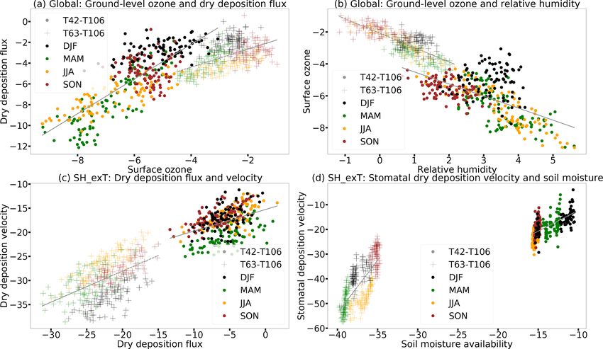
T. Emmerichs et al.: Dry deposition                                                                                                         499

       – irstom=2: variable LAI,                                    2.2.2    Cuticular deposition
       – irstom=3: T dependency and
                                                                    According to several field studies (e.g. Van Pul and Jacobs,
       – irstom=4: VPD dependency, respectively.                    1994; Hogg et al., 2007; Fares et al., 2012), cuticular depo-
  – irstom=5: all modifications.                                    sition is an important contributor to ozone uptake and should
                                                                    not be neglected in models. Therefore, an explicit parameter-
  – irstom=1: stomatal resistance with variable LAI at leaf         ization of cuticular deposition as used in many North Ameri-
    scale. Instead of choosing LAI of 1 in Eq. (5) to repre-        can air quality modelling studies (Huang et al., 2016; Kharol
    sent the stomatal resistance at leaf level, as is done by       et al., 2018) has been implemented. The gas uptake by leaf
    the original code, Eq. (5) is calculated at canopy level        surfaces is based on two parallel routes, for which an analogy
    using the actual LAI and then multiplied by LAI to ob-          to ozone (highly reactive) and sulfur dioxide (very soluble)
    tain the average stomatal resistance at leaf level. For this    is used. The cuticular resistance is calculated as
    case, the DDEP namelist parameter l_ganzeori has to be                             Rcut,d (O3 )
    set to .TRUE..                                                  Rcut (X) = −5                        ,                    (13)
                                                                                 10 · H (X) + sreac (X)
   The stomatal activity of plants and the strength of surface–     where H (X) is the effective Henry’s law coefficient as a mea-
atmosphere coupling strongly depend on the parameterized            sure of the solubility. The reactivity of a species is rated by
plant–water stress (Combe et al., 2016). The soil water bud-        the parameter sreac . For highly reactive species (sreac = 1),
get is represented by a “bucket scheme” where the soil wa-          the same property as for ozone is assumed (second term in
ter in a single layer is prescribed by a geographically vary-       Eq. 13), while for less reactive species (sreac = 0.1, 0) the
ing predefined field capacity and soil wetness governed by          uptake is effectively reduced (Wesely, 1989). For soluble
transpiration, precipitation, runoff, snow melt and drainage        species, the uptake at wet skin is assumed to be similar to
(Roeckner et al., 2003). This scheme is used by so-called           the one of sulfur dioxide and is calculated as
“first-generation” models. However, EMAC controls evapo-                                                                         −1
transpiration through the stomatal resistance (Appendix B),                             1/3                         sreac (X)
                                                                    Rws (X) =                     + 10−7 · H (X) +                      ,   (14)
which is the most important feature of biophysical (“second-                        Rcut,w (SO2 )                  Rcut,w (O3 )
generation”) land surface models. Thereby, the stomatal re-         where Rcut,w (SO2 ) and Rcut,w (O3 ) are the resistances of sul-
sistance is calculated often like the one described here (Eq. 4)    fur dioxide and ozone at wet surfaces, respectively. The con-
including temperature, VPD and soil moisture stress (Senevi-        stant values of the default formulae (Eqs. A4, A5) are re-
ratne et al., 2010; Sellers et al., 1997). The originally used      placed by parameterizations which account for the meteoro-
plant–water stress function of Jarvis (1976) and Sellers et al.     logical dependence of cuticular uptake according to Zhang
(1986), however, relies on leaf water potential (f (ψ)) for         et al. (2002):
different plant types, which is difficult to estimate. Hence,                                       Rcut,d0 (O3 /SO2 )
EMAC uses a plant–water stress function dependent on                Rcut,d (O3 /SO2 ) =                                                     (15)
soil moisture (f (Ws ). The default parameterization (Eq. A3,                           exp(0.03 · RH) · LAI0.25 · u∗
ifws = 0 in VERTEX &CTRL), applies the permanent wilt-                                  Rcut,w0 (O3 /SO2 )
                                                                    Rcut,w (O3 /SO2 ) =                    ,                                (16)
ing point of plants (Wpwp , 35 % of field capacity1 ) as a lower                           LAI0.5 · u∗
threshold in the calculation of the soil moisture stress fac-       where the cuticular resistance of O3 and SO2 , respectively,
tor (f (Ws )). However, soil moisture is significantly under-       is distinguished for dry canopies (Rcut,d ) and wet canopies
predicted by the model in some regions and the calculated           (Rcut,w ) depending on relative humidity (RH in %), LAI
f (Ws ) can be 0 for long periods. This is unrealistic and effec-   (in m2 m−2 ) and friction velocity (u∗ in m s−1 ). The in-
tively shuts down dry deposition, e.g. during the dry season        put parameters are Rcut,d0 (O3 )=5000 s m−1 , Rcut,w0 (O3 ) =
in the Amazon region. For this reason, f (Ws ) is parameter-        300 s m−1 and Rcut,d0 (SO2 ) = 2000 s m−1 (Zhang et al.,
ized here according to the original formulation by Delworth         2002). For rain and dew conditions, values of 50 s m−1 and
and Manabe (1988) by removing the lower limit:                      100 s m−1 are prescribed for Rcut,w0 (SO2 ). In contrast to tra-

              1       Ws (t) > Wcr                                  ditional approaches, these parameterizations also consider
f (Ws ) = Ws (t)                                             (12)   the aerodynamic and the quasi-laminar boundary resistances
               Wcr    Ws (t) ≤ Wcr ,
                                                                    of individual leaves. For the usage in MESSy, this can be
where Ws (t) is the surface soil wetness (in m). Wcr (in m) is      switched on via l_ganzeori=.FALSE. in the &CTRL namelist
defined as the critical soil moisture level (75 % of the field      of DDEP.
capacity) at which the transpiration of plants is reduced. The
modified parameterization in Eq. (12) can be applied by set-        2.3     Simulations
ting the &CTRL parameter ifws = in the VERTEX namelist.
                                                                    In order to answer the different research questions of this
   1 maximum amount of water the soil can hold against gravity      study, two different types of simulations have been per-
over periods of several days                                        formed (Table 1).

https://doi.org/10.5194/gmd-14-495-2021                                                        Geosci. Model Dev., 14, 495–519, 2021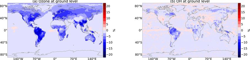
500                                                                                        T. Emmerichs et al.: Dry deposition

    1. The first kind were simulations to investigate dry depo-     the four cloud parameters have been tuned in advance ac-
       sition and the effect of the modifications in VERTEX:        cording to Mauritsen et al. (2012). The tuning factors can be
       these simulations are based on the Chemistry-Climate         found in Table 2. The radiative imbalance at TOA is slightly
       Model Initiative (CCMI) setup (Jöckel et al., 2016). To      positive at present-day conditions (Mauritsen et al., 2012;
       allow for comparison with measurements, the model dy-        Stephens et al., 2012); here, E5VDIFF gives a negative value.
       namics have been nudged towards realistic meteorology        The difference between the tuned VERTEX and E5VDIFF is
       by the assimilation of data from the European Centre for     small and within the uncertainty range of ±0.4 W m−2 .
       Medium-Range Weather Forecasts (ECMWF) (Jöckel                  Additionally, global mean values of surface temperature,
       et al., 2010). Additionally, the QCTM mode is used;          cloud liquid water, relative humidity and planetary bound-
       i.e. the chemistry does not feed back to the dynamics,       ary layer height of EMAC using E5VDIFF and EMAC us-
       resulting in the same meteorology for all simulations        ing VERTEX with the respective uncertainty range for the
       (Deckert et al., 2011). All modifications for the dry de-    period 1979–2008 are represented in Fig. 2. The results for
       position scheme are employed in a 7-year simulation          cloud liquid water and planetary boundary height show no
       (REV, 2009–2015). Additionally, a 1.5-year simulation        significant differences between the VERTEX and E5VDIFF
       covering the period 2017 to July 2018 (2017 as spin-         simulations since the annual mean of each falls in the con-
       up) has been performed to cover the measurement pe-          fidence interval of the other. This is not always the case for
       riods (Sect. 4). For the same periods, simulations with      surface temperature and relative humidity. However, the 30-
       the same configuration, except applying the default dry      year means of surface temperature and relative humidity sim-
       deposition scheme (DEF), have been conducted. The in-        ulated by E5VDIFF and VERTEX are not significantly dif-
       dividual effects of the different modifications are inves-   ferent.
       tigated by two 2-year simulations employing the dif-
       ferent namelist switches (Sect. 2.2). Moreover, a free-
       running sensitivity simulation with an additional tem-       4   Evaluation with deposition measurements
       perature and drought stress factor for evapotranspira-
       tion (Appendix B) has been performed aiming at an im-        To assess the impact of the code revision/modifications on
       proved representation of local meteorology especially        the variability of dry deposition, we compare the sensitivity
       in the Amazon. The station simulation output and the         simulations DEF, REV, REV-fTfVPD, REV-fws and REV-
       global output are analysed in Sects. 4 and 5, respec-        NNTR (see Table 1, all at T106L31 resolution) with dry de-
       tively. In addition, two 2-year simulations are realized     position measurements at four field sites (listed in Table 3).
       for different horizontal resolutions (REST42, REST63)        The chosen data sets are the best available of ozone dry de-
       to investigate the resolution dependency of dry deposi-      position (flux data and ozone mixing ratio or velocity data)
       tion (Sect. 7). All these simulations use 31 model layers    with the required temporal resolution and coverage of di-
       with the top at 10 hPa and take the first year of simula-    verse biomes of the world. The analysis is aimed at covering
       tion as spin-up.                                             the recent decade, which includes the most extreme drought
                                                                    and heat events (where the stomatal stress factors are aimed).
    2. The second kind were simulations for the evaluation of       For the reason of uniqueness and importance of atmospheric
       VERTEX as the boundary layer scheme:                         processes in a remote and pristine forest like the Amazon,
       two pure dynamical (i.e. without chemistry) 30-year          we included measurements from, among others, the Ama-
       simulations with the old (clim-E5) and the new bound-        zon Tall Tower Observatory (ATTO). Ozone dry deposition
       ary layer description (clim-VER), respectively, have         fluxes were measured with the eddy covariance and gradi-
       been performed.                                              ent method (Ontario). From these data, deposition velocities
                                                                    were calculated by the means of ozone concentration data.
All simulations were performed at the Jülich Supercomput-
                                                                    The eddy covariance technique determines a turbulent flux
ing Centre with the JURECA Cluster (Jülich Supercomput-
                                                                    by the covariance of the measured vertical velocity and the
ing Centre, 2018).
                                                                    gas concentration. Due to the stochastic nature of turbulence,
                                                                    these measurements have an uncertainty of 10 % to 20 % un-
3     VERTEX evaluation                                             der typical observation conditions (Rannik et al., 2016). For
                                                                    the gradient method used at the Borden forest research sta-
In order to advise the usage of VERTEX (with the default set-       tion, the dry deposition flux was estimated from concentra-
tings) as the default vertical exchange submodel in MESSy,          tion gradients below and above the canopy and the eddy dif-
the dynamics produced by both submodels are compared.               fusivity according to the Monin–Obukhov similarity theory.
Therefore, two dynamical, free-running 30-year simulations          The estimated dry deposition velocities (Vd ) show an uncer-
have been performed using the E5VDIFF or the VERTEX                 tainty of ≈ 20 %, which is due to the assigned canopy, the
submodels, respectively. To obtain a comparable radiative           inherent limitations of the algorithm and the measurement
imbalance at TOA (top of the atmosphere) with VERTEX,               uncertainties in concentrations. However, results are in good

Geosci. Model Dev., 14, 495–519, 2021                                                https://doi.org/10.5194/gmd-14-495-2021
T. Emmerichs et al.: Dry deposition                                                                                                    501

Table 1. List of EMAC simulations

      Simulation            Spatial resolution       Time period                    Remarks
      (1) Dry deposition mechanism: CCMI chemistry, nudged, no feedbacks (QCTM)
      REST42                T42L31 (2.8◦ × 2.8◦ )    2009/2010                      irstom=5, ifws=1, l_ganzeori=F
      REST63                T63L31 (1.9◦ × 1.9◦ )    2009/2010                      irstom=5, ifws=1, l_ganzeori=F
      REV (revised)         T106L31 (1.1◦ × 1.1◦ )   2009–2015, 2017–June 2018      irstom=5, ifws=1, l_ganzeori=F
      DEF (default)         T106L31 (1.1◦ × 1.1◦ )   2009–2015, 2017–June 2018      default ddep scheme
      REV-fws               T106L31 (1.1◦ × 1.1◦ )   2009/2010                      irstom=5, ifws=0, l_ganzeori=F
      REV-fTfD              T106L31 (1.1◦ × 1.1◦ )   2009/2010                      irstom=2, ifws=1, l_ganzeori=F
      REV-NNTR              T106L31 (1.1◦ × 1.1◦ )   2014/2015                      free-running, all ddep modifications (as REV),
                                                                                    all stress factors applied to evapotranspiration
                                                                                    (izwet=1)
      (2) Climatology comparison: no chemistry, free-running
      clim-E5               T42L90 (2.8◦ × 2.8◦ ,    1979–2008                      E5VDIFF for vertical exchange
                            up to 0.01 hPa)
      clim-VER              T42L90 (2.8◦ × 2.8◦ ,    1979–2008                      VERTEX for vertical exchange
                            up to 0.01 hPa)

Table 2. Overview of tuning parameter settings and global mean properties.

                  Parameters                                                    EMAC (E5VDIFF)        EMAC (VERTEX)
                  Cloud mass flux above level of non-buoyancy                                  0.3                   0.3
                  Entrainment rate for shallow convection                                1 × 10⁻³              1 × 10⁻³
                  Entrainment rate for deep convection                                    1 ×10⁻⁴               1 ×10⁻⁴
                  Conversion rate to rain in convective clouds                          1.5 ×10⁻⁴             1.6 ×10⁻⁴
                  Properties                                        Observed∗   EMAC (E5VDIFF)        EMAC (VERTEX)
                  Total cloud cover [%]                                                     67.12                 67.27
                  Water vapour path [kg m−2 ]                                               25.03                 24.83
                  Liquid water path [kg m−2 ]                                               0.077                 0.077
                  Total precipitation [mm d−1 ]                                              1.28                  1.31
                  Surface net shortwave [W m−2 ]                      152–167              158.27                158.32
                  Surface net longwave [W m−2 ]                      −(40–57)              −54.82                −54.93
                  Surface sensible heat flux [W m−2 ]                −(16–19)              −18.75                −19.65
                  Surface latent heat flux [W m−2 ]                  −(75–87)              −87.45                −88.73
                  Planetary albedo [%]                                                      32.38                 32.37
                  Shortwave net at TOA [W m−2 ]                       238–244              230.99                231.00
                  Longwave net at TOA [W m−2 ]                     −(237–241)             −232.46               −232.55
                  Radiation imbalance at TOA [W m−2 ]                                       −1.47                 −1.55
                ∗ Stevens and Schwartz (2012)

agreement with other eddy covariance measurements (Wu                   deposition velocity. The available micrometeorological data
et al., 2016).                                                          help to distinguish the different effects. From the hourly data,
                                                                        we calculated multiyear (2010–2012) monthly means. To ex-
4.1   Annual cycle of dry deposition                                    plore the contribution of stomatal and cuticular uptake, the
                                                                        individual velocities are calculated for O3 according to the
                                                                        model calculations (Kerkweg et al., 2006):
The annual cycle of dry deposition is mainly driven by the
evolution of vegetation and is generally represented well in
models (Silva and Heald, 2018). Here, we use the long time
series measured at Borden and Hyytiälä to identify the im-
pact of the code modifications on the annual cycle of dry

https://doi.org/10.5194/gmd-14-495-2021                                                       Geosci. Model Dev., 14, 495–519, 2021
502                                                                                        T. Emmerichs et al.: Dry deposition

Figure 2. Global mean properties and the uncertainty range (95 % confidence interval in shaded) of the climatology simulations with
E5VDIFF (clim-E5) and with VERTEX (clim-VER) for the period 1979–2008.

                                                                    mation of relative humidity leading to too-low simulated cu-
                                                                    ticular deposition (Fig. 3c, e). This effect exceeds the impact
         (1 − ws) · (1 − cvs) · veg                                 of the overestimation of relative humidity (only) in summer,
Gcut,d =
                Rcut,d (O3 )                                        because the LAI is higher in summer. In general, the cuticu-
            ws · (1 − cvs)                                          lar uptake parameterization accounting for LAI, friction ve-
  Gcut,w =                                                (17)
             Rcut,w (O3 )                                           locity, RH and surface wetness conditions performs, in our
Gns = Gcut,d + Gcut,w                                     (18)      simulations, better than parameterizations without these de-
                                                                    pendencies as expected from the study of Wu et al. (2018).
         (1 − ws) · (1 − cvs) · veg
Gstom =                                                   (19)      Unfortunately, the cuticular uptake parameterization also in-
              Rstom,corr (O3 )                                      troduces uncertainties to the modelled non-stomatal uptake.
          Gp                                                        Moreover, accounting for biogenic volatile organic com-
vp =               · vd ,                                 (20)
     Gstom + Gns                                                    pounds (BVOCs) like in Makar et al. (2017) would enhance
                                                                    in-canopy loss of ozone, significantly increase non-stomatal
where G names the individual conductances (inverse of re-           dry deposition and lead to improved simulation results (Wu
sistance) of stomata (stom), dry cuticle (cut,d), wet cuticle       et al., 2018). The representation of in-canopy air chemistry
(cut,w) and non-stomata (ns). Here, veg, ws and cvs give            is outside the scope of the present study but planned within a
the vegetation fraction, the wet skin fraction and the snow-        subsequent study.
covered fraction, respectively. Gp and vp are the individual           In contrast, the amplitude of the annual cycle and the mean
conductance and the velocity of one pathway. Further terms          of dry deposition fluxes in Hyytiälä are overestimated by
are described in Sect. 2.2.                                         both schemes during spring and summer (Fig. 3b). For the
   The multiyear (2010–2012) annual cycle of the simulated          default scheme, this is due to the oversimplification of the
dry deposition velocity at Borden forest (Fig. 3a) captures         stomatal uptake that only accounts for a constant LAI of
the observed cycle well until June. The new scheme repro-           1 m2 m−2 (see Sect. 2.2.1), which is far from the measured
duces the observations better than the old scheme. This is a        LAI of 3–4 m2 m−2 during this period (Keronen et al., 2003).
consequence of the increase in nighttime mean velocities due        Enabling the new scheme (REV), increases the dry deposi-
to the much larger cuticular contribution (Fig. B1a, b). How-       tion velocity which reproduces the measured values in au-
ever, due to the overestimated stomatal uptake in the default       tumn better. The contribution of non-stomatal dry deposition
scheme (see Sect. 2.2.1), only slight deviations from the new       of 25 %–45 % during the day reported by Rannik et al. (2012)
dry deposition scheme are visible in the daily mean shown           is represented partly by that. However, the new scheme leads
in Fig. 3a. The mismatch of the simulated and measured Vd           to an even higher overestimation by the model from April
from August to October is a consequence of the underesti-

Geosci. Model Dev., 14, 495–519, 2021                                                 https://doi.org/10.5194/gmd-14-495-2021
T. Emmerichs et al.: Dry deposition 503
to July. The sensitivity simulation REV-fws (default f (Ws ))
Table 3. Dry deposition measurements. In the description of vegetation/climate, the reported LAI (in m2 m−2 ) is given in brackets; vdmod and vdobs are the average measured and modelled points to the increase of the soil moisture stress function (see
Fares et al. (2012) and Fares et
Available on request: Matthias
Sect. 2.2.1, Eq. 12) as one reason for the overestimation of
Sörgel (m.soergel@mpic.de)
Vd in summer (Fig. 3b, f). Moreover, the overestimation in
June/July is partly (∼ 10 %) due to the too-high model LAI
Keronen et al. (2003)
compared to the measured values of 3–4 (Fig. B2a). The re-
al. (2012–2014)b
Wu et al. (2018)
maining gap (Fig. 3f) can be explained by restricting the anal-
ysis to wet conditions (RH > 70 %) only and the analysis of
Reference
the sensitivity simulation REF-fTfD (no f (T ) and f (VPD)).
This suggests that the overestimated Vd (Fig. B2c) in summer
is due to the stress factors for stomatal uptake since the mod-
elled and measured temperatures are a mismatch. VPD has
0.18 (0.67), 0.33 (1,0) been identified by Rannik et al. (2012) as a strong driver of
vdmod (vdobs ) cm s−1
daytime total deposition velocity, which confirms the impor-
tance of inclusion of VPD dependence for stomatal uptake.
0.29 (0.28)
0.22 (0.49)
0.34 (0.47)
4.2 Importance of stress factors for the diurnal
variation of deposition
Nov 2015, Apr/May 2018
The short-term measurements at Lindcove research station
and at ATTO are used to assess the impact of the stress fac-
Oct 2009–Nov 2010
tors on the diurnal cycle of dry deposition velocity in spring
and summer. Additionally, micrometeorological and addi-
Time period
2010–2012
2010–2012
tional flux data make possible to consider the stomatal re-
sistance (∼ inverse of the velocity, calculations according to
Fares et al., 2012) and the underlying meteorological con-
ditions. Since the respective micrometeorological measure-
ments are not available at ATTO, data extracted from the
61.85◦ N, 24.28◦ E (22 m/16 ma )
ERA5 global climate reanalysis at the 1000 hPa pressure
36.35◦ N, 119.09◦ W (131 m)
44.19◦ N, 79.56◦ W (33 m)
level (Copernicus, 2017) are used here.
2.15◦ S, 59.01◦ W (41 m)
The diurnal cycle of dry deposition velocity at the Lind-
cove research station follows the solar variation (Fares et al.,
Location (height)
2012) and is generally well reproduced by the model with
the best match in spring (Fig. 4). The revised dry deposition
scheme reduces the underestimation of measured nighttime
Vd due to the inclusion of cuticular uptake, which Fares et al.
(2012) identified as an important ozone sink for exactly this
measurement site. The measured dry deposition velocity in-
a Meteorological measurement height. b Ozone data are not available here.
(LAI of 3–4)/cold temperate
creases at sunrise (around 15:00 UTC) and remains almost
(LAI of 6)/tropical humid
(LAI of 3)/Mediterranean
Boreal forest, Scots Pine,
constant during the day. This is only reproduced by the re-
(LAI of 4.6)/temperate
vised dry deposition scheme. The comparison of the dry de-
Vegetation/climate
position velocity from the revised scheme (red line) and the
Citrus orchard
velocity without stomatal T and VPD stress (gray line) in
Mixed forest
Rainforest
Fig. 4a illustrates the necessity of accounting for the stress
factors. This is consistent with Fares et al. (2012), who re-
ported a high negative correlation of Vd (sto) with VPD and
temperature and related it to stomatal stress. The direct com-
Hyytiälä, southern Finland
Lindcove research station,
Borden research station,
parison of the stomatal resistances calculated from measured
(ATTO), Manaus, Brazil
dry deposition velocity.
and modelled variables (Fig. 4c) shows an improvement of
Amazon Tall Tower
the modelled resistances (comparing DEF and REV). How-
California, USA
Ontario, Canada
ever, the modelled daytime stomatal resistance is still too
(SMEAR II)
high compared to the measurements. This points to an un-
derestimation of stomatal uptake by the model during the
day. A small fraction can be explained by the direct effect
Site
of the stomatal soil moisture stress in the model which does
https://doi.org/10.5194/gmd-14-495-2021 Geosci. Model Dev., 14, 495–519, 2021
504                                                                                         T. Emmerichs et al.: Dry deposition

Figure 3. Measured (obs) and modelled (DEF, REV) multiyear mean (2010–2012) and REV-fws (2010) annual cycle. (a, c, e) Borden forest
and (b, d, f) Hyytiälä; arrows indicate 1σ .

not occur in reality since the citrus orchard was watered dur-      compared to other sites (e.g. Lindcove). The measured dry
ing the measurement campaign. Contrastingly, in summer,             deposition velocity at ATTO shown in Fig. 5a and b is no
the model underestimation of Vd is higher than in spring            exception but shows a high variability (standard deviation).
(Fig. 4b). As seen from the comparison of stomatal resistance       The diurnal cycle follows the solar radiation with maximum
values (Fig. 4d), the model underestimates the stomatal up-         Vd at 15:00 UTC and highest amplitude during the wet sea-
take. This is because the irrigation of the orchard leads to        son (April–May 2018). The amplitude of the diurnal cycle
cooling sustained evapotranspiration and keeps f (T ) low.          is highly underestimated in both EMAC simulations, with
Thus, in the model, a too-high temperature stress acts on           the highest mismatch during daytime. This is similar for
the stomata. Moreover, neglecting the soil moisture stress          other models. In fact, Hardacre et al. (2015) report a gen-
on stomata would bring the stomatal resistance values closer        eral and large underestimation of dry deposition velocities
since the irrigation at the site ensures a constant and high soil   by models over tropical forests with highest predicted values
moisture. The irrigation of the citrus orchard during the day       of 0.25 cm s−1 . Here, the simulation with the revised dry de-
also enhances surface wetness and favours deposition at cuti-       position scheme (REV) shows only a minor increase of Vd
cles (Fares et al., 2012; Altimir et al., 2006) which cannot be     during the wet season. Since stomatal uptake is known to be
captured by the model. Fares et al. (2012) estimate the stom-       an important daytime sink (Freire et al., 2017), the underes-
atal contribution to only account for 20 %–45 % of the total        timation of the total dry deposition flux is partly attributed
daytime dry deposition flux during both seasons and point to        to a too-low simulated stomatal uptake caused by the over-
soil deposition and reactions of ozone with NO and VOCs             estimation of temperature and the underestimation of rela-
as major sinks at the citrus orchard, especially during flow-       tive humidity (Fig. B3). The increase of dry deposition ve-
ering season. The contribution of these pathways is expected        locity by the new scheme is mainly due to the lowered soil
to be enhanced by the inclusion of further BVOCs within the         moisture stress on stomata (f (Ws )) shown in Fig. 5e. Freire
chemical mechanism and the explicit parameterization of in-         et al. (2017) also links stomatal uptake to the efficiency of
canopy residence and transport.                                     turbulent mixing in transporting ozone down to the canopy.
   Tropical forests are known to be effective O3 sinks with         In general, 10 % of the total ozone sink during daytime and
observed mean midday maximum dry deposition velocity of             39 % during night are associated with in-canopy processes
2.3 cm s−1 (Rummel et al., 2007) due to much higher LAI             (Freire et al., 2017). Freire et al. (2017) and Bourtsoukidis

Geosci. Model Dev., 14, 495–519, 2021                                                 https://doi.org/10.5194/gmd-14-495-2021
T. Emmerichs et al.: Dry deposition                                                                                              505

Figure 4. Diurnal cycles of measured (obs) and modelled (DEF, REV, REV-fTfD) ozone dry deposition velocity and stomatal resistance in
spring and summer 2010 at Lindcove research station.

Figure 5. Diurnal cycles of measured (obs) and modelled (DEF, REV, REV-NNTR: free-running f (T ) and f (VPD) for evapotranspiration)
ozone dry deposition velocities in wet and dry seasons at ATTO (gray: standard deviation).

https://doi.org/10.5194/gmd-14-495-2021                                                   Geosci. Model Dev., 14, 495–519, 2021
506                                                                                         T. Emmerichs et al.: Dry deposition

Figure 6. Multiyear (2010–2015) mean absolute values in boreal summer.

Figure 7. Multiyear (2010–2015) mean absolute changes in boreal summer: i.e. difference between the revised and default scheme (REV –
DEF).

et al. (2018) identified the oxidation of sesquiterpenes as an       ing stress factors for the stomata that are double the ones
important contributor to the chemical nighttime sink. Cutic-         derived from reanalysis data (Fig. 5f). This mismatch leads
ular deposition might also play a role in humid conditions           to an underestimation of stomatal uptake. This result is con-
during night (Rummel et al., 2007), which is underestimated          firmed by the sensitivity simulation REV-NNTR for which
by the model due to the biased relative humidity (Fig. 5c).          no meteorological nudging has been applied, and the stress
   The uncertainty introduced by the mismatching meteorol-           factors f (T ) and f (VPD) are also used for the calculation of
ogy becomes even more obvious when comparing measure-                evapotranspiration. The REV-NNTR simulation yields much
ments and simulations for November 2015. This month was              more realistic results compared to the measurements, captur-
characterized by temperatures of 2 to 3 degreeC above av-            ing at least 50 % of the measured Vd during the day (Fig. 5b).
erage and unusually little rainfall (compared to usual condi-        This improvement is partly due to the omission of nudging,
tions in this season) due to a strong El Niño event (National        as the latter can have a detrimental effect on precipitation
Centers for Environmental Information, 2016). The dryness            and evaporation (Jeuken et al., 1996). The temperature bias
is overestimated by the model with a too-high temperature            of the model is associated with the missing soil moisture
(1 = +5 to +8 K), too-low relative humidity (1 = −30 %               buffer simulated by the bucket scheme. Incorporating a 5-
to −40 %)) and too-dry soil. The lack of available soil mois-        layer scheme has been shown to lead to a more realistic soil
ture (f (Ws ) = 0) effectively shuts down stomatal deposition        water storage capacity, especially in the Amazon, and to a
in the default simulation (DEF), whereas the modification            removal of this bias (Hagemann and Stacke, 2013). Never-
of the soil moisture stress function (neglecting the artificial      theless, the REV-NNTR simulation suggests that the stress
lower limit; see Eq. 12) in the revised model (REV) allows           factors f (T ) and f (VPD) significantly contribute to buffer
for an increased deposition (Fig. 5b). The temperature and           soil moisture and ameliorate the dryness bias.
relative humidity biases result in corresponding mismatch-

Geosci. Model Dev., 14, 495–519, 2021                                                  https://doi.org/10.5194/gmd-14-495-2021
T. Emmerichs et al.: Dry deposition                                                                                                    507

Figure 8. Mean changes (2010) of dry deposition velocity in boreal summer. (a) f (Ws ) modification; (b) temperature and VPD stress.

                                                                          Concerning the stomatal deposition, the impacts of three
                                                                       different stress factors are considered. First, over relatively
                                                                       dry soil, i.e. where soil moisture exceeds 35 % of field ca-
                                                                       pacity (wilting point of plants), the soil moisture stress is
                                                                       reduced by the modified parameterization. Neglecting the
                                                                       plants’ wilting point as the lower limit for soil moisture stress
                                                                       on stomata weakens the dependency on field capacity. Thus,
                                                                       dry deposition is enhanced by up to 0.32 cm s−1 , as illus-
                                                                       trated in Fig. 8a. Second, the inclusion of temperature and
                                                                       (third) VPD adjustment factors, indeed, leads to a spatially
                                                                       varying impact of ±0.27 cm s−1 change in Vd (Fig. 8b). In
                                                                       humid and cold temperate regions, like Siberia and Canada,
Figure 9. Relative change [%] and absolute change [Tg yr−1 ] (num-
                                                                       no temperature stress appears and the VPD adjustment fac-
bers on bars) of annual global loss by dry deposition of O3 , SO2 ,    tor increases the stomatal uptake. In the eastern US, Kaza-
HNO3 and HCHO (REV – DEF).                                             khstan and central Amazon during boreal summer, stomata
                                                                       are stressed by temperature and VPD. This effect is overpre-
                                                                       dicted by the model, as the humidity over the Amazon forest
                                                                       is probably too low in the model (see Fig. B3). The stress
5   Global impact on ground-level ozone
                                                                       factors are shown in Fig. B4c and d.
                                                                          However, the overall decrease in ozone concentration
Given the importance of dry deposition for ground-level                dampens the impact of the change in dry deposition flux.
ozone and the uncertainty of dry deposition parameteriza-              In total, the changes by the revised dry deposition scheme
tions in models (Young et al., 2018; Hardacre et al., 2015),           increase the multiyear mean (2010–2015) loss of ozone by
the global impact of the implemented code changes is as-               dry deposition from 946 to 1001 Tg yr−1 (Young et al., 2018;
sessed in this section. The global (boreal) summer mean dis-           Hu et al., 2017). Accordingly, (boreal) summer ground-level
tributions of deposition velocity and ground-level mixing ra-          ozone over land is reduced by up to 12 ppb (24 %), peaking
tio for O3 shown in Fig. 6a–b are generally in the same range          over Scandinavia, Asia, central Africa and eastern Canada
as reported for global models (e.g. Val Martin et al., 2014;           (Fig. 7b). In the Northern Hemisphere, also the zonal mean
Hardacre et al., 2015). However, like most global models,              of the tropospheric ozone mixing ratio show a noticeable re-
EMAC overestimates tropospheric ozone in comparison to                 duction far from the ground compared to the default scheme
satellite observations (Righi et al., 2015). Applying the re-          (Fig. 11a). This has the potential to reduce the positive bias
vised dry deposition scheme increases the mean summer Vd               of tropospheric ozone on the Northern Hemisphere (20 %) re-
by up to 0.5 cm s−1 (Fig. 7a). The highest fraction of this in-        ported by Young et al. (2018). However, besides ozone, also
crease arises from the inclusion of cuticular uptake at wet            other atmospheric tracer gases are affected by the change in
surfaces (Vcut,w ) (Fig. B4b). The effect is large over the most       dry deposition. The global annual dry deposition flux of odd
northern continental regions (Fig. 7d) and even more pro-              oxygen (Ox )2 , which includes many important tropospheric
nounced where LAI is high like in Scandinavia and eastern              trace gases, increases from 978 to 1032 Tg yr−1 due to the
Canada (for LAI distribution, see Fig. B4a). Additionally,             revision. This is in good agreement with the reported num-
the uptake at dry surfaces (Vcut,d ) is enhanced with up to            bers by Hu et al. (2017) and Young et al. (2018). In Fig. 9,
0.3 cm s−1 higher dry deposition velocity (Fig. 7c). This is
because the default scheme applies a very high constant re-              2 O ≡ O+O +NO +2NO +3N O +HNO +HNO +BrO+
                                                                            x      3     2      3  2 5 3   4
sistance for this process.                                             HOBr + BrNO2 + 2BrNO3 + PAN

https://doi.org/10.5194/gmd-14-495-2021                                                      Geosci. Model Dev., 14, 495–519, 2021
508 T. Emmerichs et al.: Dry deposition
Figure 10. Relative change of multiyear (2010–2015) mean at ground level (DEF – REV).
Figure 11. Relative change of multiyear (2010–2015) zonal mean (DEF – REV).
we show additionally the absolute and relative change of the 6 Uncertainties in modelling stomatal conductance
multiyear annual average dry deposition loss of SO2 , NO2 ,
HNO3 and HCHO. As a very soluble species, the loss of SO2
is increased by the revised dry deposition scheme, whereas Dry deposition is a highly uncertain term in modelling ozone
the predefined low cuticular and wet skin resistance of HNO3 pollution (Young et al., 2018; Clifton et al., 2020a). Its repre-
in the old scheme were replaced with the new mechanism, sentation is generally limited by a lack of measurements and
leading to an decrease in dry deposition. The altered loss of process understanding but also to a large extent driven by
NO2 and HCHO and other ozone precursors at ground level, the quality of land cover information (Hardacre et al., 2015;
especially soluble oxygenated VOCs, contributes to the total Clifton et al., 2020b). Although the dry deposition scheme by
change in ozone loss. NO2 is deposited almost 40 % more Wesely (1989) is commonly used in global and regional mod-
significantly, contributing to the net reduction in ozone pro- els (e.g. MOZART, GEOS-Chem), the approach has some
duction but is mostly counterbalanced by other processes. constraints (Hardacre et al., 2015). The disadvantage of the
The change of HCHO dry deposition flux is small on a global big-leaf approach used in MESSy is that a vertical varia-
and annual scale and only important regionally, mostly in tion of leaf properties, affecting, for instance, the attenua-
(boreal) summer, when it decreases HCHO at ground level tion of solar radiation, is not considered (e.g. Clifton et al.,
(Fig. 12b) by up to 25 %. Thereby, the change in wet up- 2020b). Regarding stomatal uptake, we neglect the meso-
take is highest but is partially counterbalanced by other ef- phyll resistance as reactions inside the leaf are commonly
fects. This leads to lower HO2 production from HCHO pho- assumed to not limit stomatal ozone uptake, whereas, be-
tooxidation and lower NO-to-NO2 conversion and thus lower sides mostly supporting laboratory studies (e.g. Sun et al.,
ozone production (Seinfeld and Pandis, 2016). These effects 2016), a few contradicting findings exist (e.g. Tuzet et al.,
also impact the OH mixing ratio (Figs. 10b, 11b) which con- 2011). The here-used empirical multiplicative algorithm by
trols the methane lifetime predicted by the model. However, Jarvis (1976) for stomatal modelling has one general draw-
for a clearer effect, a longer simulated time period would be back concerning that the environmental responses to stom-
needed. A detailed analysis of the trace gas budgets is be- ata are treated clearly in contrast to experimental evidence
yond the scope of this paper and will be investigated in a (Damour et al., 2010). However, Jarvis-type models have
subsequent study. been shown to be able to compete with the semi-mechanistic
Anet − gs models which link stomatal uptake to the CO2 as-
similation during plant photosynthesis (Fares et al., 2013; Lu,
2018). The critics in Fares et al. (2013) state that the Jarvis
Geosci. Model Dev., 14, 495–519, 2021 https://doi.org/10.5194/gmd-14-495-2021T. Emmerichs et al.: Dry deposition 509
Figure 12. Relative change of multiyear (2010–2015) boreal summer mean (DEF – REV).
model cannot capture the afternoon depression of ozone dry spatial resolutions: 2.8◦ × 2.8◦ , 1.9◦ × 1.9◦ and 1.1◦ × 1.1◦
deposition is due to the original used VPD stress factor which (REST42, REST63, and REV (T106) in Table 1).
has been replaced here by a mechanistic one based on the op- In Fig. 14a, the resolution dependency is shown for the
timized exchange of CO2 and water by plants (Katul et al., annual dry deposition flux of ozone on different continen-
2009). Furthermore, a larger set of land cover types is ex- tal regions. The annual dry deposition fluxes differ by up to
pected to improve the vegetation-dependent variation of dry 40 Tg yr−1 globally between the different resolutions, with
deposition. The parameters used to model dry deposition of highest dry deposition at high resolution (T106). For the
stomata, cuticle and soil are biome dependent and using gen- Northern Hemisphere (and consequently globally), this dif-
eralized ones like for the input cuticular resistance can lead ference is driven by the higher annual mean ground-level
to differences in dry deposition (Hoshika et al., 2018). Exem- ozone compared to the lower resolutions (Fig. 14c). How-
plary discrepancies for the stomatal conductance calculated ever, this effect cannot be disentangled from the effect of de-
with different parameter sets are shown in Fig. 13 as the sum- creased dry deposition velocity on ground-level ozone. Glob-
mer mean of 2010. Thereby, the temperature stress factor has ally, increasing differences in O3 are anti-correlated with rel-
been calculated as in Eq. (6) using the obtained surface tem- ative humidity as shown in Fig. 15a (ρ = −0.8). The impact
perature by EMAC (Fig. 13a, c) and applied to the model of humidity on ozone chemistry is considered to be relatively
(DEFAULT) stomatal conductance (Eq. 17) with two differ- weak (Jacob and Winner, 2009), but Kavassalis and Murphy
ent parameter sets for coniferous and mixed forest by Simp- (2017) showed for the US that only dry deposition establishes
son et al. (2012)3 and Zhang et al. (2003)4 . Jarvis (1976) ob- the observed anti-correlation between ozone and relative hu-
tained the parameters from a set of measurements in mixed midity. A dominating positive correlation of the dry deposi-
hardwood/coniferous forest in Washington. In general, the tion flux with the velocity only occurs on the Southern Hemi-
parameters are related to measurements where the absolute sphere extratropics (SH_exT), which is highest between T63
values are influenced by multiple factors like genotype and and T106 (Fig. 15c). This can be attributed to discrepancies
local climatic conditions (Sulis et al., 2015; Tuovinen et al., in stomatal deposition (Fig. 15d) driven by differences in hu-
2009; Hoshika et al., 2018). So, for global modelling, mostly midity which might be caused by different moisture cycles
simplified parameters have to be used like in the European and transpiration.
Monitoring and Evaluation Programme (EMEP) (Simpson
et al., 2012).
8 Conclusion and recommendations
7 Sensitivity to model resolution
Dry deposition to the Earth’s surface is a key process for
The simulation of dry deposition depends on meteorology in- the representation of ground-level ozone in global models.
cluding boundary layer processes, radiation (cloud distribu- Its parameterizations constitutes a relevant part of the model
tion and reflectivity) and ozone chemistry as well as on input uncertainty (Hardacre et al., 2015; Wu et al., 2018). Revis-
fields like vegetation density (LAI) (Jones, 1992). Model hor- ing the dry deposition scheme of EMAC leads to an im-
izontal resolution inherently affects the amplitude and dis- proved representation of surface ozone in regions with a pos-
tribution of (regridded) surface processes and the artificial itive model ozone bias (e.g. Europe). The highest increase in
dilution of ozone precursors that are emitted. This aspect is ozone dry deposition is due to the implementation of cutic-
investigated here by analysing simulations at three different ular uptake whose contribution is important especially dur-
ing night over moist surfaces. The extension of the stom-
3 Used parameters: T ◦ ◦ ◦ atal uptake with temperature and VPD adjustment factors ac-
min = 0 C, Topt = 18 C, Tmax = 36 C.
4 Used parameters: T ◦ ◦ ◦ counts for the desired link of plant activity to hydroclimate
min = −3 C, Topt = 21 C, Tmax = 42 C.
https://doi.org/10.5194/gmd-14-495-2021 Geosci. Model Dev., 14, 495–519, 2021You can also read