Limitations of assuming internal mixing between different aerosol species: a case study with sulfate geoengineering simulations - ACP ...
←
→
Page content transcription
If your browser does not render page correctly, please read the page content below
Research article
Atmos. Chem. Phys., 22, 1739–1756, 2022
https://doi.org/10.5194/acp-22-1739-2022
© Author(s) 2022. This work is distributed under
the Creative Commons Attribution 4.0 License.

             Limitations of assuming internal mixing between
            different aerosol species: a case study with sulfate
                        geoengineering simulations
            Daniele Visioni1 , Simone Tilmes2 , Charles Bardeen2 , Michael Mills2 , Douglas G. MacMartin1 ,
                                       Ben Kravitz3,4 , and Jadwiga H. Richter5
              1 SibleySchool of Mechanical and Aerospace Engineering, Cornell University, Ithaca, NY, USA
                            2 Atmospheric Chemistry, Observations, and Modeling Laboratory,

                               National Center for Atmospheric Research, Boulder CO, USA
               3 Department of Earth and Atmospheric Sciences, Indiana University, Bloomington, IN, USA
               4 Atmospheric Sciences and Global Change Division, Pacific Northwest National Laboratory,

                                                    Richland, WA, USA
        5 Climate and Global Dynamics Laboratory, National Center for Atmospheric Research, Boulder, CO, USA

                             Correspondence: Daniele Visioni (daniele.visioni@cornell.edu)

                                  Received: 11 August 2021 – Discussion started: 17 August 2021
                         Revised: 5 January 2022 – Accepted: 6 January 2022 – Published: 4 February 2022

      Abstract. Simulating the complex aerosol microphysical processes in a comprehensive Earth system model
      can be very computationally intensive; therefore many models utilize a modal approach, where aerosol size
      distributions are represented by observation-derived lognormal functions, and internal mixing between different
      aerosol species within an aerosol mode is often assumed. This approach has been shown to yield satisfactory
      results across a large array of applications, but there may be cases where the simplification in this approach may
      produce some shortcomings. In this work we show specific conditions under which the current approximations
      used in some modal approaches might yield incorrect answers. Using results from the Community Earth System
      Model v1 (CESM1) Geoengineering Large Ensemble (GLENS) project, we analyze the effects in the troposphere
      of a continuous increasing load of sulfate aerosols in the stratosphere, with the aim of counteracting the surface
      warming produced by non-mitigated increasing greenhouse gas (GHG) concentrations between 2020–2100. We
      show that the simulated results pertaining to the evolution of sea salt and dust aerosols in the upper troposphere
      are not realistic due to internal mixing assumptions in the modal aerosol treatment, which in this case reduces
      the size, and thus the settling velocities, of those particles and ultimately changes their mixing ratio below the
      tropopause. The unnatural increase of these aerosol species affects, in turn, the simulation of upper tropospheric
      ice formation, resulting in an increase in ice clouds that is not due to any meaningful physical mechanisms. While
      we show that this does not significantly affect the overall results of the simulations, we point to some areas where
      results should be interpreted with care in modeling simulations using similar approximations: in particular, in
      the evolution of upper tropospheric clouds when large amounts of sulfate are present in the stratosphere, as after
      a large explosive volcanic eruption or in similar stratospheric aerosol injection cases. Finally, we suggest that
      this can be avoided if sulfate aerosols in the coarse mode, the predominant species in these situations, are treated
      separately from other aerosol species in the model.

Published by Copernicus Publications on behalf of the European Geosciences Union.
1740                            D. Visioni et al.: Limitations of assuming internal mixing between different aerosol species

1   Introduction                                                 tual size distribution of the aerosols can be represented by
                                                                 the combination of multiple lognormal functions with fixed
A comprehensive representation of aerosol processes in           standard deviations that are based on observations. Further-
Earth system models is crucial for a variety of reasons.         more, a modal approach to aerosol microphysics must also
Aerosols are one of the main short-term forcing agents in        make assumptions about the internal and external mixing of
the climate system, and uncertainties in the estimate of their   aerosol species (Fassi-Fihri et al., 1997): internal mixing is
overall forcing effects are still quite large (Boucher et al.,   defined as the modeling of an aerosol particle as a mixing of
2013). Directly, they scatter incoming solar radiation, thus     the constituent species (Clarke et al., 2004), either as a ho-
influencing surface temperatures, and they also absorb both      mogeneous mix or as a coated sphere containing a solid core
solar radiation and outgoing planetary radiation, locally in-    and coated by a liquid exterior. More simply put, it assumes
creasing air temperatures, modifying circulation patterns and    that different species of aerosols in every grid box are present
affecting meteorology. Indirectly, they affect the climate by    in the same proportion, and that their physical characteris-
modifying cloud cover, acting as cloud condensation nuclei       tics can be described by the same average size distribution.
(CCN) and ice nuclei (IN), and changing clouds’ physical         External mixing is defined as the treatment of particle pop-
and radiative properties (also through local atmospheric heat-   ulations as composed of different species with distinct com-
ing). Lastly, once they are deposited to the surface, they af-   positions, and no assumption needs to be made with regards
fect land and ice albedo through the melting of snow and ice.    to the localized proportion of the various species, as they are
Aerosols at the surface also contribute to air pollution (es-    treated differently (Riemer et al., 2019). Some discussion and
pecially via particulate matter (PM) below 2.5 and 10 µm in      comparisons of the application of sectional and modal micro-
diameter, Ayala et al., 2012) and may affect soils and ecosys-   physics modules in climate models can be found in Weisen-
tems through acid deposition (Vet et al., 2014).                 stein et al. (2007), Kokkola et al. (2009), Kleinschmitt et al.
   Atmospheric aerosols may have different sizes, ranging        (2017), and more specifically for sulfate geoengineering ap-
from 0.001 to 100 µm in diameter, and their characteristics      plications in Laakso et al. (2022).
(number concentration, mass, shape, chemical composition            A modal treatment of aerosols in climate models has been
and other physical properties) may change through emis-          shown to successfully reproduce aerosol measurements for
sion (from natural or anthropogenic sources), nucleation (de-    various events. In this work, in particular, we focus on the
fined as the formation of new particles), coagulation (defined   Community Atmosphere Model version 5.0 (CAM5) and
as the combination of existing aerosol particles, decreasing     its implementation in the Community Earth System Model
their number concentration but leaving the overall mass un-      (CESM), using the Modal Aerosol Module with three modes
altered), condensational growth of chemical species in va-       (MAM3, Liu et al., 2012). This approach has been shown
por form (such as H2 SO4 , NH3 , HNO3 and volatile organ-        to correctly reproduce tropospheric aerosols in a baseline
ics gases) on existing particles, gas-phase and aqueous-phase    climate (see Liu et al., 2012; Samset et al., 2014), and
chemistry, water uptake (Ghan and Zaveri, 2007) and their        also to correctly reproduce the evolution of the stratospheric
removal through gravitational settling (dry deposition), in-     sulfate aerosol layer in the extreme case of explosive vol-
cloud scavenging (defined as the removal of aerosol parti-       canic eruptions (Robock, 2000), as detailed by Mills et al.
cles by precipitation particles) and below-cloud scavenging      (2016, 2017) for the Whole Atmosphere Community Cli-
(defined as the capture of aerosol particles by precipitating    mate Model (WACCM) version of CESM1, with a high top
droplets, Feng, 2009). They can, of course, be composed of       (140 km) and 70 vertical layers. This model has been used
different chemical species: the main components are usu-         for climate simulations of stratospheric aerosol intervention
ally sea salt, mineral dust, black carbon, organic matter, ni-   (SAI), a form of climate engineering that has been proposed
trate, ammonium and sulfate. Wang et al. (2020) provide a        (Budyko, 1969; Crutzen, 2006) as a way to temporarily re-
recent overview of all aerosol-related processes: this list of   duce global surface temperatures by mimicking the cool-
processes can give an idea of how challenging it can be to       ing effect of volcanic eruptions through injecting SO2 in
represent aerosol processes correctly in climate models, both    the stratosphere. In both the case of volcanic eruptions and
due to the uncertainties in each process and in their combi-     for the proposed artificial injections, once SO2 reaches the
nation, and because of the high computational burden nec-        stratosphere, it oxidizes, eventually forming gaseous H2 SO4 ,
essary to correctly reproduce the known parts of each pro-       which then either nucleates, forming new sulfate aerosol par-
cess. For this reason, most processes need to treat aerosols     ticles of H2 SO4 -H2 O, or condenses onto existing particles
in parametrized ways with different complexities, ranging        (already existing particles could also coagulate, resulting in
from the least (bulk model, considering all aerosols as de-      larger particles with the same overall mass). While this pro-
scribed by a single mean radius and standard deviation) to       cess transforms all SO2 into aerosols with an e-folding time
the most complex (sectional model, considering a large num-      of around 1 month (Mills et al., 2017), the produced aerosols
ber of “bins” of different sizes for each species where the      tend to remain in the stratosphere for 1 year or more (Vi-
aerosols can grow or shrink). An intermediate approach is        sioni et al., 2018b), and are removed through large-scale
the modal method: it works on the assumption that the ac-        stratospheric circulation, which moves them poleward, or by

Atmos. Chem. Phys., 22, 1739–1756, 2022                                           https://doi.org/10.5194/acp-22-1739-2022
D. Visioni et al.: Limitations of assuming internal mixing between different aerosol species                                  1741

gravitational settling or stratosphere–troposphere exchange,           In this study, as an example to illustrate some of the short-
crossing the tropopause. Once in the troposphere, they are          comings of the modal aerosol treatment in MAM3, we use
quickly removed through dry or wet deposition (Kremser              the GLENS simulations to explore the effects of a large
et al., 2016).                                                      amount of sulfate aerosols in the stratosphere on tropospheric
   Climate engineering simulations with CESM1(WACCM)                aerosol concentrations and on cirrus ice cloud formation in
in the Geoengineering Large Ensemble (GLENS; Tilmes                 CESM1(WACCM). We will briefly describe how aerosol
et al., 2018a) have shown that it would be possible to              microphysics and cirrus ice formation are parameterized in
maintain global surface temperatures at 2010–2029 levels            Sect. 2, then discuss how aerosols in the upper troposphere
even under a scenario where emissions of greenhouse gases           change in the simulations of interest in Sect. 3 and discuss
(GHGs) continue unabated by increasing the amount of SO2            how that affects upper tropospheric ice in Sect. 4. Finally,
injected throughout the century. This technique may be able         possible radiative effects at the top of the atmosphere of the
to reduce some of the harmful climatic effects produced by          identified changes will be discussed in Sect. 5.
temperature increase (Tilmes et al., 2018a; Kravitz et al.,
2019), by reducing the amount of incoming sunlight, but             2     Model description
it would not be a perfect solution. In fact, the atmosphere
and surface would be impacted in various ways by the pro-           In this section we will briefly describe the simulations used
duced aerosols, for example, the chemical composition of the        in this work, and then describe the components of the model
stratosphere and the dynamical response produced by the lo-         that will be of use in our analysis.
cal stratospheric heating (Richter et al., 2017; Tilmes et al.,        The Geoengineering Large Ensemble (GLENS, Tilmes
2018b), which in turn can influence precipitation (Simpson          et al., 2018a) is an ensemble of simulations performed with
et al., 2019) and the high-latitude seasonal cycle of temper-       CESM1 (WACCM), with all simulations using surface emis-
ature (Jiang et al., 2019). Once the aerosols are deposited         sions from the Representative Concentration Pathway 8.5
to the surface they may also affect soils; however, consider-       (RCP) scenario. Twenty-one ensemble members are avail-
ing the much larger amount of tropospheric sulfate aerosols         able for the period 2010–2030 under RCP8.5 (hereafter,
produced by both natural and human activities, those settling       termed Baseline). From each of these, in 2020 a scenario
from the stratosphere would have a marginal impact every-           is simulated where SO2 is injected at four locations: 30◦ N
where except in some pristine areas (Visioni et al., 2020b).        and S, with injections at 23 km altitude, and 15◦ N and S at
Other processes that may be affected by SAI include aerosol         25 km altitude. Each year, an algorithm (described by Kravitz
interactions with cirrus clouds, which are a key component          et al., 2017) determines the amount of SO2 to be injected
of the radiation balance. Water clouds at lower altitudes have      at each location in order to maintain the mean surface tem-
a net cooling effect because they reflect solar radiation (see      perature, the inter-hemispheric surface temperature gradient,
for instance Yi et al., 2017); on the other hand, the effect of     and the Equator-to-pole temperature gradient at their 2020
cirrus clouds made of ice crystals and produced in the upper        values in the presence of growing greenhouse gas concentra-
troposphere by supercooled water particles is harder to de-         tions. All the simulations of SAI are extended to 2100 (here-
termine, but is widely understood to be positive (i.e., it pro-     after, termed GLENS), and four ensemble members of the
duces a net warming at the surface; Fusina et al., 2007) due        Baseline cases (without SAI) are run to the at least the year
to their trapping of outgoing planetary radiation. Kuebbeler        2097. Please note that, compared to the original simulations
et al. (2012) and Visioni et al. (2018a) found in two differ-       described in Tilmes et al. (2018a), one more ensemble mem-
ent climate models (ECHAM-HAM5 and ULAQ-CCM, us-                    ber is available for both GLENS and Baseline (from 20 to 21
ing a modal and a sectional aerosol approach, respectively)         and from 3 to 4, respectively).
that the change in the vertical temperature gradient resulting
from the stratospheric heating would reduce the formation of
                                                                    2.1    The Modal Aerosol Model in CESM
tropical cirrus ice clouds by less than 10 %, thus contribut-
ing to surface cooling. This effect is tied to the fact that, in    The Modal Aerosol Model (MAM) was first described by Liu
both models, the amount of water vapor reaching the upper           et al. (2012), where it was evaluated for tropospheric aerosol
troposphere and which is necessary for cloud formation is di-       loads. Some modifications have been made to include in-
rectly tied to the available turbulent kinetic energy, which is a   teractive stratospheric aerosols, described in depth by Mills
function of the vertical temperature gradient, and is therefore     et al. (2016), therein validated in the case of the Pinatubo
a purely dynamical effect. Cirisan et al. (2013) on the other       1991 eruption.
hand investigated the possible microphysical effect of the in-         For CESM1(WACCM) climate simulations, the three-
creased sulfate load on cirrus cloud formation, but found no        mode version (MAM3) is used, with aerosol species divided
significant impact due to the much larger size of the aerosols      in three different lognormal modes of fixed width, named
from the stratosphere compared to those already present in          Aitken (dry diameter size range between 0.015 and 0.05 µm),
the troposphere due to other activities.                            accumulation (between 0.05 and 0.3 µm) and coarse mode
                                                                    (between 0.80 and 3.65 µm; all estimates from Liu et al.,

https://doi.org/10.5194/acp-22-1739-2022                                            Atmos. Chem. Phys., 22, 1739–1756, 2022
1742                              D. Visioni et al.: Limitations of assuming internal mixing between different aerosol species

2012), going from the smallest to the largest. Sulfate parti-       in CESM1(WACCM), the Community Atmospheric Model
cles can grow by condensation (from H2 SO4 vapor condens-           version 5 (CAM5), both processes are present and we will
ing on existing particles, locally maintaining particle num-        briefly describe both below.
bers but increasing mass) or coagulation (locally reducing             The process of homogeneous freezing is based on the as-
particle numbers but maintaining mass). When, by either pro-        sumption that only sulfate particles in the Aitken mode work
cess, the tail of the distribution of the particles in one of the   as ice nuclei (IN), using the portion of the Aitken mode par-
modes grows to a size that would nominally be in the size           ticles with radii greater than 0.1 µm (Liu and Penner, 2005;
range for the larger mode, the particles are transferred to the     Liu et al., 2007). Other works have used all available sul-
larger mode. This is done, as detailed by Easter et al. (2004),     fate modes for homogeneous freezing (Shi et al., 2015), and
by defining a lower and upper limit for the dry diameter in         this would clearly affect the results. The process of homo-
each mode, and transferring part of the local number concen-        geneous freezing is assumed to happen only when clouds are
tration to the larger mode when the threshold is surpassed.         present, together with a probability distribution from Kärcher
In the stratosphere the sulfate particles can also shrink due       and Burkhardt (2008) that determines when the supersatu-
to evaporation, thus allowing for a coarse-to-accumulation          ration is above the threshold for homogeneous freezing to
mode transfer.                                                      happen. This means that homogeneous freezing can happen
   Compared to the more computationally demanding MAM               only when local vertical velocities are high (Kärcher and
version with seven aerosol modes (MAM7), in MAM3 all                Lohmann, 2002). Those velocities are determined following
aerosol species are considered to be internally mixed within        Morrison and Pinto (2005) as
each of the three modes, thus sharing composition and size                  r
distribution. The mass for the single species has to be con-                   2
                                                                    wsub =       TKE,                                          (1)
served, both globally and locally, and thus can only change                    3
in each grid box if particles are moved from one grid box           with the turbulent kinetic energy (TKE) determined using a
to another, either because of air mass movement or because          steady state energy balance as in Bretherton and Park (2009).
of gravitational settling or other tropospheric removal pro-           For heterogeneous freezing, only coarse mode dust parti-
cesses. Liu et al. (2012) justify this approach by noting           cles are assumed to be available IN (although the exclusion of
that the sources of different aerosol types are geographi-          soot particles and other particles as inefficient ice nuclei has
cally separated and thus unlikely to affect each other in the       been debated; see Kärcher and Burkhardt, 2008). Given the
simplified version used for long-term climate applications.         internal mixing assumption in MAM3, the number of avail-
Coarse mode sulfate aerosols are, in quiescent conditions,          able dust nuclei is determined as a fraction of the overall
also scarce in the troposphere: in the AeroCom multi-model          amount of coarse mode particles given the mass of dust and
mean (Textor et al., 2006) they were determined to be less          the overall aerosol mass
than 2 % of all sulfate aerosols, with a preponderance of par-
                                                                                md

ticles in the accumulation mode in the troposphere. The as-         Nd =                × Nc ,                                   (2)
                                                                             md + mss
sumption by Liu et al. (2012) would therefore hold in the
background atmosphere. We will show in the next section             where md is the mass of dust in the coarse mode, mss is
that the presence of the coarse mode sulfate particles pro-         the mass of sea salt in the coarse mode and Nc is the to-
duced by SAI fundamentally breaks this assumption, unnat-           tal number of particles in the coarse mode. This approach
urally modifying the size and quantity of non-sulfate aerosol       assumes a negligible amount of coarse mode sulfate in the
species in the upper troposphere.                                   upper tropical stratosphere in the denominator of the frac-
                                                                    tion. Another shortcoming of the heterogeneous freezing de-
2.2    The formation of cirrus ice clouds in CESM
                                                                    scription in this version of WACCM, as already discussed by
                                                                    Mills et al. (2017), is that when heterogeneous freezing oc-
Cirrus clouds play an important part in the radiation budget,       curs, IN that have nucleated to form ice particles are not re-
but have generally been poorly represented in general circu-        moved from the available reservoir, thus allowing too many
lation models (GCMs) for a variety of reasons, among them           particles to be formed via heterogeneous freezing.
a poor horizontal resolution which fails to capture the scale          This approach to the microphysical modeling of cirrus
needed to represent some of the processes and a large spread        clouds in CESM has been discussed recently by Maloney
in the ice water content simulated by models (Jiang et al.,         et al. (2019), who compared it with a more complex approach
2012). There are two processes that can produce ice crys-           using the coupled Community Aerosol and Radiation Model
tals in the upper troposphere: homogeneous nucleation of            for Atmospheres (CARMA) sectional scheme, and compared
ice crystals from sulfate aerosols and heterogeneous immer-         both with measurements from the National Aeronautics and
sion freezing of mineral dust. Normally, homogeneous freez-         Space Administration Airborne Tropical Tropopause Exper-
ing is assumed to be the dominant process, although there           iment (ATTREX 3) and with observations from the Cloud-
are instances where this is not the case (Knopf and Koop,           Aerosol Lidar with Orthogonal Polarization (CALIOP) on-
2006; Cziczo et al., 2013). In the atmospheric model used           board the CALIPSO satellite. They found that while the

Atmos. Chem. Phys., 22, 1739–1756, 2022                                              https://doi.org/10.5194/acp-22-1739-2022
D. Visioni et al.: Limitations of assuming internal mixing between different aerosol species                                   1743

CAM5 approach was capable of correctly representing the            the tropopause clearly visible as a change in concentration.
annual average cloud fraction profile in the tropics (20◦ N        Nonetheless, the average concentration of sulfate under SAI
to 20◦ S), it tended to underrepresent the cirrus fraction in      is much larger even in the upper troposphere (Fig. 1b) and
the tropical tropopause layer. Similar results were also previ-    only returns close to the Baseline levels close to the surface,
ously found by Bardeen et al. (2013).                              where other sulfate sources are predominant (Fig. 1c).
                                                                      Figure 1 also shows the behavior of dust and sea salt in
                                                                   the coarse mode in the same altitude–latitude region (those
3   Simulated tropospheric aerosols                                are the only other aerosol species considered in this version
                                                                   of CESM1 in the coarse mode: black carbon is only found
The geographical distribution of tropospheric aerosols in          in the accumulation mode). Various behaviors can be found
the unperturbed atmosphere depends mainly on the sur-              depending on the altitude of analysis for the GLENS case.
face sources of the aerosols or aerosol precursors; once the       We focus here on the uppermost troposphere, right below
aerosols are produced in the atmosphere or are directly emit-      the tropopause (black boxes in Fig. 1), and on a layer be-
ted, they can be affected by long range transport, upward          low, in the upper troposphere (green boxes). In the upper
currents and sediment through gravitational settling or scav-      level, both dust (Fig. 1f) and sea salt (Fig. 1j) present be-
enging. An in-depth analysis of sources and sinks of atmo-         havior that is much more similar to that of sulfate: a large,
spheric aerosols can be found, for instance, in Lamarque           initial increase in concentration in the first 5 to 10 years fol-
et al. (2010). We focus here on sulfate, dust and sea salt,        lowed by either a constant evolution or by a small decrease
as their changes will be of interest when analyzing the ef-        (from 0.1 to 0.2 µm kg−1 for dust in the upper layer; from
fects on cirrus formation. Sulfate particles are mostly formed     0.06 to 0.2 µm kg−1 and from 0.9 to 0.17 µm kg−1 for sea
through surface emission of SO2 , which can be oxidized to         salt in the upper and lower layer). Only dust in the lower
form sulfuric acid and then sulfate particles by condensa-         layer (Fig. 1g) does not show such an abrupt initial increase.
tion in the smaller (Aitken) mode. For this reason, coarse         On the other hand, in the Baseline case, the dust mixing ra-
mode sulfate particles near the surface are much less fre-         tios show a decrease by 25 % over the 80 years of analysis in
quent than dust or sea salt, as shown in Fig. 1a as compared       the lower level. There is no immediate physical mechanism
to Fig. 1e and i. For the latter two, their concentration de-      by which such changes could be observed in aerosol species
creases with increasing altitude as the scavenging processes       independent of sulfate; therefore, a more in-depth analysis is
reduce their number, whereas there is an additional sulfate        necessary.
layer in the stratosphere (the Junge layer), discovered and           One possible explanation would be a change in the sur-
discussed by Junge et al. (1961). This happens because of the      face emissions of these species. However, the vertical pro-
presence of various sources of sulfate aerosols in the strato-     files of tropical concentrations for the three species seem to
sphere, even without considering volcanic aerosols from ex-        exclude this (Figs. 1d, h, l and 3). This is further confirmed
plosive volcanic eruptions. In particular, surface emissions of    by the analysis of the overall burdens shown in Fig. 2. For
carbonyl sulfide (OCS) and dimethyl sulfide (DMS), which           these, no initial abrupt change can be identified, and the time
are light, well-mixed gases that may reach the stratosphere        evolution shows the opposite behavior from that found in
where they are oxidized, forming sulfate aerosols (Vet et al.,     Fig. 1, with a minor reduction in GLENS compared to Base-
2014). Meteoric sulfur also plays a part in the formation of       line. The behavior of the Baseline case is consistent with
the layer (see Gómez Martín et al., 2017). The quantity of         previous projections: Mahowald and Luo (2003) predicted
sulfate aerosols produced in the stratosphere with an arti-        a reduction in overall dust emissions with increasing GHGs
ficial injection of SO2 would be larger by some orders of          due to higher precipitation and more surface moisture pro-
magnitude than the amount in the quiescent Junge layer. The        duced by the warmer air; thus the precipitation decrease in
full stratospheric distribution in the case of GLENS has been      GLENS (Cheng et al., 2019) would exacerbate differences
described elsewhere (i.e., Kravitz et al., 2019), so here we       between dust burden in GLENS and the Baseline. Struthers
simply report that at 50 hPa, between 30◦ N and 30◦ S, the         et al. (2013) on the other hand projected a small increase in
average mass concentration for the last 20 years of simula-        sea salt aerosols mostly as a result of increased surface wind
tion is 163 µg kg−1 , compared to 0.4 µg kg−1 in the unper-        speeds. Having excluded that changes in surface emissions
turbed case; while this simulation considered high cooling         are the cause of the abrupt increase identified, we further in-
(∼ 4 ◦ C reduction in global mean temperature), even much          vestigate the smaller aerosol modes (Fig. 3). In this case, we
smaller amounts of SAI would lead to substantially more            see a much closer agreement of the values in GLENS to those
stratospheric sulfate than the unperturbed case. This magni-       of the initial Baseline conditions for sea salt and dust: this in-
tude is driven by the long lifetime of the produced aerosol        dicates that the initial aim of the GLENS simulations, which
particles in the stratosphere (around 12 months, Visioni et al.,   was to maintain the state of the climate as close as possible
2018b). Once the particles cross the tropopause, the various       to 2010–2029 conditions, also helps with not modifying sur-
removal processes strongly reduce the lifetime, driving the        face emission sources of those species. The time evolution of
concentration down. This is visible already in Fig. 1a, with       the globally averaged quantities for these species and modes

https://doi.org/10.5194/acp-22-1739-2022                                           Atmos. Chem. Phys., 22, 1739–1756, 2022
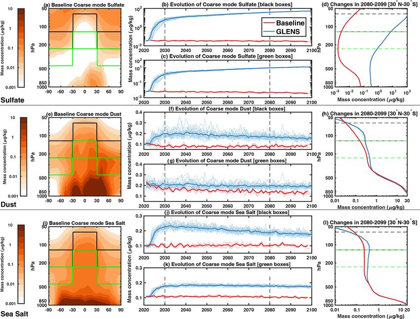
1744                                 D. Visioni et al.: Limitations of assuming internal mixing between different aerosol species

Figure 1. Mass concentration (in micrograms per kilogram of air) of coarse mode species (sulfate, top row; dust, middle row; and sea salt,
bottom row). On the left, panels (a), (e) and (i) indicate the Baseline (2020–2029) zonal mean concentration for the respective species, with
the black and green boxes indicating the areas considered in the averages for the central panels (b, c, f, g, i, k). The uppermost limit of the
green boxes and the lowermost limit of the black boxes coincide. Panels (b), (f), (j) and (c), (g) and (k) for each species show the annual
evolution of the concentration in the black (b, f, j) and green (c, g, k) boxes, with thinner lines showing the single ensemble realizations,
and the thicker lines show the ensemble mean; red lines indicate the Baseline simulations, while blue lines indicate the GLENS simulations.
Black dashed lines in panels (b), (f), (j) and (c), (g) and (k) indicate the periods of analysis for panels (a), (e), (i) and (d), (h) and (l),
respectively. On the right, panels (d), (h) and (l) show the vertical profiles in both cases (Baseline in red, and GLENS in blue) for the period
2080–2099. The black lines in panels (d), (h) and (l) indicate the altitude of analysis in panels (b), (f) and (j), while the green lines indicate
the altitude of analysis in panels (c), (g) and (k).

also does not show the same abrupt change as that found in                 (Fig. 1 for the vertical distribution, and Fig. 2 for the spa-
Fig. 1 (see Figs. S1 and S2 in the Supplement). So, clearly                tial distribution). The parameterization requires that in each
the cause of the rapid change in concentration of the coarse               grid box, all aerosols in one mode are treated as the same in
mode must be the result of the very rapid increase in SO4                  terms of their size distribution, so for each mode, only one
aerosol concentration, by more than 4 orders of magnitude.                 mode diameter and one number concentration are used in the
   The solution to this conundrum can be found by analyzing                online calculations (since the geometric standard deviation
the behavior of the simulated radius of the particles in the               is constant throughout the atmosphere). The mass concen-
three modes (Fig. 4). In MAM3, all aerosol species within an               trations of the different species are then calculated using a
aerosol mode are assumed to be internally mixed. The simpli-               reference density for each species (Liu et al., 2012). This in-
fied assumption that different aerosols peak at different loca-            formation is necessary to calculate the gravitational settling
tions in the lower atmosphere is reasonable for the Baseline               velocities (at each layer), which follow Seinfeld and Pandis

Atmos. Chem. Phys., 22, 1739–1756, 2022                                                        https://doi.org/10.5194/acp-22-1739-2022

D. Visioni et al.: Limitations of assuming internal mixing between different aerosol species                                       1745

Figure 2. Zonally averaged total column burden of dust (a) and sea salt (c) (considering all modes) in 2010–2029 (red dashed line), 2080–
2099 in Baseline (red line) and 2080–2099 in GLENS (blue line). Evolution of the globally integrated dust (b) and sea salt (d) burden
(Tg yr−1 ). Thinner lines show the single ensemble realizations, while the thicker lines show the ensemble mean.

(2016), where the equation of a free-falling spherical particle        already present in the upper troposphere. Due to the small
in a fluid that has reached terminal velocity (which is done           amount of coarse mode aerosols there, and due to the in-
in less than 1 × 10⁻⁶ for particles of diameter of ' 1 µm) is          ternal mixing assumption in MAM3, the dust and sea salt
shown to be                                                            aerosols already present are “forced” to reduce in size (and to
                       1/2                                           conserve mass and to increase in number concentration; see
           4gDp Cc ρp                                                  Fig. S3). This produces a drop in the overall size by around
vt =                           ,                              (3)
             3CD ρ                                                     25 % within 3 years in the upper troposphere. Because of the
                                                                       strong dependence of gravitational settling velocities on size,
where Dp is the diameter of the particle, ρp is the density            the result is a drop in these velocities that, for dust aerosols,
of the particle, Cc is the slip-correction factor that accounts        can be estimated to be over 40 %. This is not a direct out-
for non-continuum effects (dependent on the diameter of the            put of the model, but we estimate it from Eq. (3) using the
particles) and CD is the empirical drag coefficient (dependent         approach of Seinfeld and Pandis (2016). The clear drop in
on the Reynolds number Re ).                                           vt can then explain the initial identification of the increase
   The initially identified changes can thus be explained as           in non-sulfate aerosol species: reducing settling deposition
follows. The SO4 formed in the stratosphere is the predom-             abruptly directly affects the concentration by decreasing re-
inant form of aerosols in the stratosphere, determining the            moval, especially in regions where contributions from below
radius of the particles at those altitudes. Most of these parti-       are scarce. And the reason why this is only visible in the
cles are in the coarse mode and therefore change the radius            upper troposphere is that, further below, the preponderance
considered by the model in those grid boxes. Once the sul-             of pre-existing, background coarse mode aerosol reduces the
fate aerosols cross the tropopause (whether by gravitational           strength of this effect, not changing the radii. The prepon-
settling, mostly in the tropics, or by large-scale circulation,
at higher latitudes) they are added to the particle distribution

https://doi.org/10.5194/acp-22-1739-2022                                               Atmos. Chem. Phys., 22, 1739–1756, 2022
1746 D. Visioni et al.: Limitations of assuming internal mixing between different aerosol species
Figure 3. Mass concentration (in micrograms per kilogram of air) of sulfate, dust and sea salt in the Aitken (smallest) mode and accumulation
(intermediate) mode, between 30◦ N and 30◦ S. Thinner lines show the single ensemble realizations, while the thicker lines show the ensemble
mean.
derance of other removal mechanisms (in-cloud scavenging) stratosphere) and when eventually looking at surface effects.
also reduces the effect of the gravitational settling changes. We show in this section, however, that their change does
influence the simulation of ice cloud formation in the up-
per troposphere. Visioni et al. (2021) showed that some no-
4 Effect on cirrus cloud formation ticeable changes in cloud cover are present in the GLENS
simulations, and that when separating the contribution of
We have shown that the simulated changes in dust
different types of clouds, most of these changes were at-
and sea salt in the upper troposphere in GLENS using
tributable to changes in high clouds, which are defined in
CESM1(WACCM) are non-physical in nature. However, by
CESM1(WACCM) as all clouds formed between altitudes of
looking at the concentration of the same species in the Base-
400 and 50 hPa. Furthermore, these changes were not as no-
line conditions it is clear that the overall presence of these
ticeable in other simulations performed where the same cool-
aerosols at the altitudes of analysis is small, and therefore
ing as GLENS was achieved using a solar constant reduction
would have a negligible effect both when looking at the di-
approach, or where the stratospheric heating produced by the
rect effects (for instance, on the radiative fluxes, which would
aerosols was imposed without the presence of the aerosol
be overshadowed by the effects of the sulfate aerosols in the
Atmos. Chem. Phys., 22, 1739–1756, 2022 https://doi.org/10.5194/acp-22-1739-2022D. Visioni et al.: Limitations of assuming internal mixing between different aerosol species 1747 Figure 4. Wet radius (in microns) of all three modes in the Baseline case ([2010–2029], a–d) and in GLENS ([2080–2099], e–h). (g) Vertical distribution of aerosol size in all three modes between 30◦ N and 30◦ S. Black boxes in panels (c)–(f) indicate the average area analyzed for panel (h), where the temporal evolution in Baseline (red) and GLENS (blue) is shown. Thinner lines show the single ensemble realizations, while the thicker lines show the ensemble mean. (i) Estimate of the changes in gravitational settling velocities following Seinfeld and Pandis (2016). themselves. This points towards a contribution to the changes Koop, 2006). Due to the difficulties in measuring the amount in high cloud cover in GLENS by some effects connected to of ice crystals in the upper troposphere, and due to the chal- the aerosol themselves. In particular, this points to changes in lenges of representing the processes in models, there are the freezing processes that produce ice crystals in the upper plenty of uncertainties over the predominance of one forma- troposphere, given that at those altitudes there is much less tion process over the other. In CESM, only sulfate particles in water than in the lower troposphere, and most of it is in the the Aitken mode can act as the substrate over which homoge- form of ice rather than liquid droplets (see Fig. S5). neous freezing can take place; this is generally understood to As we detailed in Sect. 2.2, there are two types of pro- be correct, as too large particles would be increasingly harder cesses that may lead to the formation of ice crystals at those to freeze (Chen et al., 2000). Since Aitken mode particles do altitudes: the spontaneous freezing of small aqueous sulfate not change in GLENS (see Fig. 3a), related changes in ho- droplets at high relative humidity rates (Chen et al., 2000), mogeneous freezing can be excluded, as already predicted known as homogeneous freezing, and the freezing of water by Cirisan et al. (2013). However, changes in homogeneous droplets mediated by the presence of insoluble aerosol par- freezing may happen as a result of dynamical changes in ticles (ice nuclei, IN), known as heterogeneous nucleation the local vertical velocities that determine the amount of wa- (Diehl and Wurzler, 2004), which can happen at lower rela- ter vapor in the upper troposphere. Since the processes that tive humidity conditions and higher temperatures (Knopf and determine those local vertical velocities happen at a much https://doi.org/10.5194/acp-22-1739-2022 Atmos. Chem. Phys., 22, 1739–1756, 2022
1748                              D. Visioni et al.: Limitations of assuming internal mixing between different aerosol species

smaller scale compared to the resolution of climate mod-           lations from GLENS. Therefore, a complete analysis is not
els, they are usually parameterized in climate models as a         possible using the whole ensemble and time period. Noting
function of vertical stability (see Eq. 1). Both previous stud-    that the main, unexplained processes (with our current un-
ies analyzing the response of ice clouds in a SAI scenario,        derstanding of ice formation) happen in the very first decade
Kuebbeler et al. (2012) and Visioni et al. (2018a), used cli-      of the simulations, for the following analysis we have re-run
mate models with a similar parameterization as CESM, and           the first 21 years of one of the ensemble members with the
found a reduction in ice cloud coverage because the warming        same configuration (thus, bit-by-bit, the result is the same)
of the stratosphere, combined with a cooling of the surface,       but retain information related to the two different upper tro-
produced a reduction in vertical temperature gradients and         pospheric freezing processes. The results in Fig. 6 confirm
thus in the turbulent kinetic energy used to determine the ve-     our previous observations. For homogeneous freezing, very
locities. A similar process can then be expected in CESM.          few changes are initially observable at any latitude, whereas
Lastly, there is no physical reason why SAI would change           large, abrupt changes are observable in the concentration of
heterogeneous freezing in ice clouds. However, given what          what the model considers to be IN for heterogeneous freez-
we identified in the previous section related to dust aerosols     ing in the first few years. This increase is much larger than the
in the upper troposphere, an influence on freezing processes       increase in the coarse mode dust aerosols identified in Fig. 1,
cannot be excluded.                                                where the overall concentration was doubled, while here the
   In Fig. 5, we show an analysis of the changes in the amount     increase is much larger, at more than 10 times the amount in
of ice in clouds under GLENS. Two particularly different be-       the first 2 years. To partially explain this change, we refer to
haviors can be noted when separating the effects at low lat-       the equation used by the model to determine the fraction of
itudes (30◦ N–30◦ S) versus the effects noted elsewhere. At        the available dust in the coarse mode, which is used as IN
low latitudes, the dynamical changes produced by the dif-          for heterogeneous freezing (Eq. 2). The available number of
ferent vertical stabilities dominate, resulting in a slow de-      dust particles that can be used by the model depends on the
crease in ice concentration in line with predictions discussed     overall amount of coarse mode particles, but it is weighted by
by Kuebbeler et al. (2012) and Visioni et al. (2018a), which       the local fraction of aerosol comprised of dust to that com-
is not a surprise, considering the very similar parameteriza-      prised of sea salt. This formula (which in normal conditions
tion of sub-grid vertical velocities. At higher latitudes, where   gives satisfactory results; see Maloney et al., 2019) presumes
there are fewer changes in the vertical temperature gradient       a lack of sulfate in the upper troposphere. In our case how-
(since the stratosphere warms much less; see Richter et al.,       ever, as we have shown, the amount of coarse mode sulfate
2017), the predominant effect is the sudden increase in IN,        is actually by far preponderant in the upper troposphere. So
resulting from the simplified aerosol treatment in the coarse      while the number of coarse mode particles Nc grows (see
mode. The increase in ice formation that the model “sees”          Fig. S3), the fraction of all aerosols that is considered does
is therefore not physical in origin, but simply an artifact of     not. This is a separate, but similar, problem as the one noted
the microphysical parameterization and thus should not be          regarding the behavior of the aerosols. We tested how sensi-
treated as a physical side effect of SAI. A clue as to the two     tive this assumption is by performing an identical simulation
different mechanisms at play can be determined by observ-          to the one that gave us information about homogeneous and
ing the rate of change at low versus high latitudes. At low        heterogeneous freezing, but modified the code so that Eq. (2)
latitudes, the changes happen gradually as the stratospheric       becomes
sulfate load (and thus the warming) increases. At high alti-
                                                                                    md

tudes, the in-cloud ice changes are very abrupt, much more         Nd =                         × Nc ,                           (4)
                                                                             md + mss + ms
similar to the aerosol changes identified previously in this
work. Further confirmation can be derived by observing the         thus correctly accounting for the mass of sulfate when con-
differences between the full GLENS simulations and the sim-        sidering the fraction of locally present coarse mode particles
ulations described by Visioni et al. (2021) with stratospheric     comprised of dust aerosols. We show the results of these sen-
heating imposed, but no aerosols. By comparing the two (see        sitivity simulations in Fig. 6 using dotted lines: as expected,
bottom panels of Fig. 5), the effect of the presence of the        this does not change the homogeneous freezing processes,
aerosols can be separated from the dynamical ones, and in-         but it does change the amount of heterogeneous IN, and re-
deed this confirms the different nature of the ice changes,        duces the non-physical increase in cloud ice identified in
since the two simulations (aerosols plus stratospheric heating     Fig. 5 at high latitudes.
and stratospheric heating alone) show no differences at low
latitudes, whereas they are as different as GLENS-Baseline         5   Radiative effects
at high latitudes.
   Further information would be gained by observing the            Here we investigate whether the changes shown in the pre-
changes in heterogeneous versus homogeneous freezing in            vious section produce some signal in the modeled radiative
these simulations. However, the output fields that separate        fluxes at the top of the atmosphere, as that would be impor-
the two processes have not been saved in the original simu-        tant in determining the effect’s significance. To do so, we use

Atmos. Chem. Phys., 22, 1739–1756, 2022                                              https://doi.org/10.5194/acp-22-1739-2022
D. Visioni et al.: Limitations of assuming internal mixing between different aerosol species 1749
Figure 5. Baseline concentration of cloud ice number concentration (a, number of particles per cm−3 ) and fractional occurrence (b) for the
period 2010–2030. In panels (c)–(e) and (f)–(h), the yearly evolution of the differences between GLENS and Baseline (in the 2010–2030
period, as for the panels above) are shown for the three latitudinal boxes separately. In the small bottom panels, the effects of the changes
produced by the aerosols are isolated by plotting the difference between GLENS and the simulations with surface cooling and stratospheric
heating but no aerosols.
the method suggested by Ghan (2013) to separate both the with the radiation (1FD ) can be defined as
direct radiative effect of the aerosols and the effect of cloud
changes produced by the aerosols. This is possible here as the 1FD = FGLENS
ALL − FGLENS
CLEAN
radiative output of CESM is both comprised of the full radia-
tive fluxes (FALL ) at the top of the atmosphere (TOA), which − FBASELINE
ALL − FBASELINE
CLEAN , (5)
consider all effects from aerosols, clouds and atmospheric
composition, and comprised of the diagnosed Clear Sky ra- and the forcing produced by the changes in clouds (1C) can
diative fluxes (where the radiative transfer model calculates be defined as
the radiative fluxes as if no clouds were present, FCLEAR ),
Clean Sky radiative fluxes (where the radiative fluxes are 1F = FGLENS GLENS
CLEAN − FCLEAN,CLEAR
calculated as if no aerosols were present, FCLEAN ) and their
combination (FCLEAN,CLEAR ). This allows for the separation − FBASELINE
CLEAN − FBASELINE
CLEAN,CLEAR . (6)
of the contributions of the added aerosols and their effects for
both the longwave (LW) and shortwave (SW) components: As Ghan (2013) notes, normally these fluxes are just an es-
the direct forcing produced by the aerosols direct interaction timation of the real components of the forcing, as to prop-
erly estimate them it would be necessary to keep the sur-
face and tropospheric temperatures fixed between the two
cases in order to avoid changes in the radiative emissions
https://doi.org/10.5194/acp-22-1739-2022 Atmos. Chem. Phys., 22, 1739–1756, 20221750 D. Visioni et al.: Limitations of assuming internal mixing between different aerosol species Figure 6. Evolution of the occurrence of homogeneous freezing in clouds (a), the concentration of what the model considers to be IN for homogeneous freezing (Aitken mode sulfate) (b) and the concentration of IN for heterogeneous freezing (coarse mode dust) (c) in GLENS in the first 21 years of simulation, for the three latitudinal bands already considered in Fig. 5. On the right, a column mean of between 50 and 400 hPa is considered (thick lines), together with the case described in the text with a sensitivity test for Eq. (2) (dotted lines). In panel (f) the ice number concentration shown in Fig. 5 is compared with that of the sensitivity experiment. of the troposphere, which would be at different temperatures in the shortwave (implying a cooling), as it reflects incoming in the two cases. In our case, however, the GLENS simu- sunlight, and positive in the longwave (implying a warming), lations have been performed on purpose to maintain simi- as it absorbs and re-emits longwave radiation, with an overall lar global surface temperatures as the Baseline 2010–2030 negative effect, as expected. We show the latitudinal break- period; some small regional temperature differences are still down of the fluxes in Fig. 7b–c normalized by the strato- present (Tilmes et al., 2018a), but overall these can be con- spheric aerosol optical depth (AOD) produced by the SO2 sidered a minor factor and the estimated forcing can be con- injections for the initial period (we pick 2026–2035 to avoid sidered to be quite robust if we always compare the radia- the very first few years when the algorithm that determines tive fluxes against the 2010–2030 period. In the case of cloud the SO2 injections is still converging; see Kravitz et al., 2017) changes, this further ensures that we are not counting effects and the last 20 years (2081–2100). A partial non-linearity can produced by the surface warming, which might also locally be identified between the two periods. This can be explained modify cloud cover. by the slight increase in stratospheric sulfate aerosol during In Fig. 7 we show the global evolution of 1FD and 1C in the whole period of analysis (see Visioni et al., 2020a; the GLENS. The aerosol direct radiative effect is linear: negative effective radius in the stratosphere in GLENS grows from Atmos. Chem. Phys., 22, 1739–1756, 2022 https://doi.org/10.5194/acp-22-1739-2022
D. Visioni et al.: Limitations of assuming internal mixing between different aerosol species                                             1751

Figure 7. Global mean evolution of TOA radiative fluxes in the LW (orange), SW (green) and Net (black) for the forcing directly produced
by the aerosols 1FD (a) and by the clouds as changed by the presence of the aerosols (1C) (d). In panels (b)–(c) and (e)–(f), respectively,
the latitudinal breakdown of the global fluxes in two periods (2026–2035 and 2081–2100) is shown for the various components. To the right
of each panel, the global mean in the considered period is shown with a triangle of the same color, and the value is given on the right. Thinner
lines show the single ensemble realizations, while the thicker lines show the ensemble mean.

0.4 to over 0.5 µm as a result of the increasing injection rates          When tropical ice clouds start decreasing because of the dy-
resulting in more coagulation of SO2 with pre-existing par-               namical mechanism produced by stratospheric heating, the
ticles). Larger aerosols scatter slightly less efficiently, but           positive bump is erased by negative forcing (less ice clouds,
they absorb more LW radiation. The changes in upper tro-                  more LW radiation escaping to space) already analyzed by
pospheric aerosols described earlier do not influence these               Visioni et al. (2018a). This is further confirmed by the latitu-
radiative fluxes, as they are, in proportion, negligible com-             dinal breakdown of 1C in Fig. 7e–f, where the (normalized
pared to the stratospheric increase. Looking at the 1C fluxes,            by stratospheric AOD) forcing in the LW goes from positive
however, we can see that the behavior of the LW 1C shows a                in the first 10 years to negative in the last 20 years.
very different behavior compared with the SW. This effect is
positive in the first ' 30 years, and then negative afterwards,           6    Conclusions
whereas the SW forcing is always positive. The SW forcing
is easily explainable as directly connected to the presence of            In this work we have identified the presence of some weak-
the aerosols above: if less sunlight reaches the troposphere,             nesses in the three-mode modal approach (MAM3) used in
because it is partially reflected in the stratosphere, the same           CESM1(WACCM) when a large amount of aerosols settles
clouds would appear to be less reflective, and hence the pos-             down from the stratosphere, as under stratospheric sulfate
itive sign of the SW (cloud masking). This does not apply to              aerosol injection, which results in some artificial changes
the LW, as globally the surface temperatures are the same, but            to cirrus clouds. MAM3 only separates the species in three
can be explained by noting that the main contributor to LW                modes depending on their size, by treating all aerosol species
trapping by clouds is upper tropospheric ice (Fusina et al.,              as the same (internal mixing assumption). When a large
2007). Since, in the first decades, mid-latitudinal ice clouds            amount of sulfate is produced (mostly in the coarse mode,
increase as shown in Fig. 5 because of “more” dust aerosols               the largest mode) in the stratosphere following the injection
acting as IN, they would trap more outgoing LW radiation.                 of SO2 in large quantities, the particles slowly descend upon

https://doi.org/10.5194/acp-22-1739-2022                                                    Atmos. Chem. Phys., 22, 1739–1756, 2022
1752                              D. Visioni et al.: Limitations of assuming internal mixing between different aerosol species

the troposphere, where they are quickly removed. However,           in a separate coarse mode that is not internally mixed with the
the size of the coarse mode particles is different (smaller)        other species compared (dust, sea salt, black carbon, etc.).
compared to that of the coarse mode particles already present       A similar approach has already been used to include an ad-
in the troposphere, whose source is at the surface. Therefore,      ditional primary carbon mode in MAM4 (Liu et al., 2016)
MAM3 “sees” an abrupt decrease in all aerosol sizes in each         in order to account for processes that affect the microphys-
grid box in the upper troposphere for the coarse mode, re-          ical properties of primary carbonaceous aerosols in the at-
sulting in smaller settling velocities for aerosol species that     mosphere. There are various applications where this obser-
would not be otherwise affected in the real world. This effect      vation might be useful: SAI is one example, but the simu-
results in an increase in the mass of particles of all species      lation of explosive volcanic eruptions is another case where
at those altitudes, even if there were no natural causes. The       it could be useful. For instance, Schmidt et al. (2018) used
effect is small, and its direct effect on the cooling produced      the same CESM1(WACCM) model described here to esti-
by the stratospheric aerosols is negligible. However, the un-       mate the global volcanic radiative forcing in the last 45 years,
natural addition of dust in the upper troposphere results in        and made a similar observation as that in this paper, but
more particles that the model can use as solid ice nuclei for       did not find an explanation. The mechanism that produced,
the freezing of ice particles in clouds. This effect is particu-    in their simulations, an increase in ice particles in the up-
larly evident at mid- and high latitudes, where the low rela-       per troposphere is definitely the same we have encountered
tive humidity and lack of aerosols make other ice formation         here, and would explain some of the LW forcing changes
processes more scarce in normal conditions. The formation           diagnosed in their simulations with a similar method (see
of these ice crystals, as simulated by the model, indeed pro-       Figs. 4 and 5 in Schmidt et al., 2018). More generally, it
duces a noticeable change in the cloud forcing, especially          would be crucial to properly represent the upper troposphere
in the first years, when the effect from the incorrect pres-        in the case of volcanic eruptions to verify their influence on
ence of the dust aerosols is large compared to other, dynam-        ice clouds as observed by some studies of the observational
ical effects that tend to reduce the amount of ice crystals in      record (see for instance Friberg et al., 2015). Future model-
the upper troposphere when a warming of the stratosphere is         ing efforts aimed at better understanding the climatic effect
present.                                                            of volcanic eruptions, such as the Volcanic Model Intercom-
   Given the setup of the GLENS experiments, this effect is         parison Project (Clyne et al., 2021) or the Interactive Strato-
counteracted by the presence of the algorithm that determines       spheric Aerosol Model Intercomparison Project (Timmreck
how much SO2 is needed every year to counteract the effect          et al., 2018), should take this into account and consider how
of the increased emissions in RCP8.5: even if the radiative         that might affect some of their results, since models with sim-
imbalance were to be large, the algorithm would just pre-           ilar modal approaches are present in both.
scribe more SO2 to be injected, therefore resulting, overall,          Lastly, this observation would also be crucial in studies
in the same global mean temperatures as if the error in the ice     that aim to combine sulfate injections with the artificial seed-
cloud formation was not there. In the sensitivity simulations       ing of upper tropospheric ice clouds with solid nuclei in or-
produced for Sect. 4, which reduced the amount of ice clouds        der to increase the size of the ice crystal and make them
incorrectly formed by the model, the cumulative amount in-          sediment faster (cloud seeding, Gasparini et al., 2020). Cao
jected in the first 20 years was 131 Tg SO2 (6.2 Tg SO2 yr−1 ),     et al. (2017), for instance, proposed a combination of the two
whereas the same period in the default simulation had a cu-         methods to stabilize global temperatures and precipitation.
mulative amount of 154 Tg SO2 (7.3 Tg SO2 yr−1 ). Consid-           Such simulations, performed with CESM1(WACCM) or any
ering that, aside from the change in Eq. (2), the two sim-          model with a similar microphysical approach, would not give
ulations were otherwise the same; we can assume that this           meaningful results. Our study shows that more care should
difference arises from the changes in ice clouds as simulated       be given to make sure that the climate models used for sim-
by the model. Overall then, if we assume this effect is con-        ulating sulfate geoengineering applications are not applied
stant throughout the whole simulation period, it would ac-          outside of the parameters for which the models give reli-
count for a cumulative injected 88 Tg SO2 over the entire           able answers. Most of the time, models are also compared
century. While this amount might seem large, it accounts            against volcanic events to make sure they properly simulate
for less than 2 years of anthropogenic emissions of SO2 at          results, but not every effect is immediately visible in those
present (Visioni et al., 2020b). This, furthermore, assumes a       cases as compared to long-term geoengineering simulations,
very large injection to overcome a considerable amount of           and a comparison of cloud changes after a volcanic eruption
warming (over 4◦ ) over the entire century. More moderate           may be complicated by various factors (Friberg et al., 2015).
mitigation scenarios would require far less cumulative injec-
tions of SO2 (for instance, see Tilmes et al., 2020).
   This does not imply that the effect can be ignored, but sug-     Data availability. All simulations analyzed in this work are
gests that going forward when using a modal approach to             available online. All GLENS simulations data are available at
aerosol microphysics, simulations where large amount of sul-        https://doi.org/10.5065/D6JH3JXX (Tilmes et al., 2018c). Data
fate is present in the stratosphere should treat sulfate aerosols   from the stratospheric heating simulations used for Fig. 5 are avail-

Atmos. Chem. Phys., 22, 1739–1756, 2022                                                https://doi.org/10.5194/acp-22-1739-2022
You can also read


