Long-period variability in ice-dammed glacier outburst floods due to evolving catchment geometry
←
→
Page content transcription
If your browser does not render page correctly, please read the page content below
The Cryosphere, 16, 333–347, 2022
https://doi.org/10.5194/tc-16-333-2022
© Author(s) 2022. This work is distributed under
the Creative Commons Attribution 4.0 License.

Long-period variability in ice-dammed glacier outburst floods due
to evolving catchment geometry
Amy Jenson1,2 , Jason M. Amundson2 , Jonathan Kingslake3 , and Eran Hood2
1 Departmentof Mathematical Sciences, Montana State University, Bozeman, Montana 59717, USA
2 Departmentof Natural Sciences, University of Alaska Southeast, Juneau, Alaska 99801, USA
3 Lamont-Doherty Earth Observatory, Columbia University, Palisades, New York 10964, USA

Correspondence: Amy Jenson (amyjenson@montana.edu)

Received: 10 May 2021 – Discussion started: 11 June 2021
Revised: 20 November 2021 – Accepted: 1 December 2021 – Published: 25 January 2022

Abstract. We combine a glacier outburst flood model with          1   Introduction
a glacier flow model to investigate decadal to centennial
variations in outburst floods originating from ice-dammed
marginal basins. Marginal basins can form due to the retreat      Glacier outburst floods (also referred to as jökulhlaups) are
and detachment of tributary glaciers, a process that often re-    sudden releases of water from ice-dammed or moraine-
sults in remnant ice being left behind. The remnant ice, which    dammed lakes. There has been a recent increase in the size
can act like an ice shelf or break apart into a pack of ice-      and number of glacial lakes due to deglaciation (e.g., Clague
bergs, limits a basin’s water storage capacity but also exerts    et al., 2012; Shugar et al., 2020; Mölg et al., 2021), raising
pressure on the underlying water and promotes drainage. We        concerns about the hazards that these lakes pose to down-
find that during glacier retreat there is a strong, nearly lin-   stream communities and infrastructure. More accurate esti-
ear relationship between flood water volume and peak dis-         mates of flood magnitude and timing may help mitigate risk
charge for individual basins, despite large changes in glacier    in areas where these hazards exist (e.g., Vincent et al., 2010;
and remnant ice volumes that are expected to impact flood         Werder et al., 2010). In addition, outburst floods cause semi-
hydrographs. Consequently, peak discharge increases over          regular but short-lived perturbations to downstream ecosys-
time as long as there is remnant ice remaining in a basin,        tems by rapidly changing sediment and nutrient concentra-
and peak discharge begins to decrease once a basin becomes        tions and proglacial water temperatures (e.g., Neal, 2007;
ice-free. Thus, similar size outburst floods can occur at very    Kjeldsen et al., 2014; Meerhoff et al., 2019). The largest of
different stages of glacier retreat. We also find that the tem-   these floods create major erosional features during glacial pe-
poral variability in outburst flood magnitude depends on how      riods (e.g., Larsen and Lamb, 2016; Keisling et al., 2020);
the floods initiate. Basins that connect to the subglacial hy-    smaller, more frequent outburst floods are also important in
drological system only after reaching flotation depth yield       driving landscape change (e.g., Russell et al., 2006; Cook
greater long-term variability in outburst floods than basins      et al., 2018; Carrivick and Tweed, 2019). Here, motivated
that are continuously connected to the subglacial hydrologi-      by observations from Mendenhall Glacier, Alaska, we focus
cal system (and therefore release floods that initiate before     on glacier outburst floods from ice-dammed marginal basins,
reaching flotation depth). Our results highlight the impor-       which form following the thinning, detachment, and retreat
tance of improving our understanding of both changes in           of tributary glaciers and often contain remnant ice left behind
basin geometry and outburst flood initiation mechanisms in        during deglaciation (e.g., Capps et al., 2010; Kingslake and
order to better assess outburst flood hazards and their impacts   Ng, 2013a; Kienholz et al., 2020) (Fig. 1).
on landscape and ecosystem evolution.                                The theory of ice-dammed outburst floods is based on the
                                                                  consideration of mass, momentum, and energy balances of
                                                                  water flowing through the subglacial drainage system (e.g.,
                                                                  Rothlisberger, 1972; Nye, 1976; Fowler, 1999; Kingslake,

Published by Copernicus Publications on behalf of the European Geosciences Union.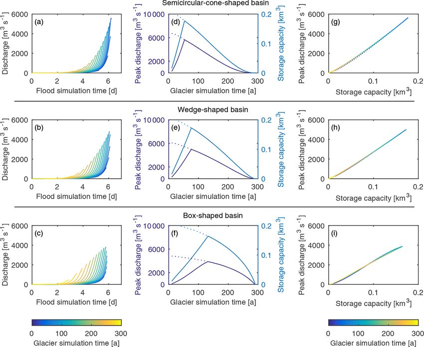
334                                          A. Jenson et al.: Long-period variability in ice-dammed glacier outburst floods

Figure 1. Repeat photos of Mendenhall Glacier, Alaska, taken in (a) 1893 (Ogilvie, 1893) and (b) 2018 (courtesy of Christian Kienholz).
Suicide Basin formed in the early 2000s when Suicide Glacier detached from Mendenhall Glacier. Annual outburst floods now originate
from Suicide Basin, which contains remnant ice from Suicide Glacier.

2013; Kessler and Anderson, 2004; Stubblefield et al., 2019;          the water pressure equals the overburden pressure of the ice
Schoof, 2020). Many outburst flood models are based on                dam, which occurs at the lake level referred to as flotation
the assumption of a circular or semicircular channel (e.g.,           depth (Thorarinsson, 1953). When an outburst flood initi-
Nye, 1976; Fowler, 1999; Kingslake, 2013); others allow               ates due to the basin reaching flotation depth, water floats
for more complex drainage configurations such as multiple             the ice dam and flows beneath the ice (1) forming a chan-
lakes in a connected hydrological system (e.g., Stubblefield          nel, (2) enlarging an existing channel, or (3) propagating a
et al., 2019) or a system of linked cavities (e.g., Kessler and       subglacial sheet of water toward the terminus (e.g., Flow-
Anderson, 2004; Schoof, 2020), which may be more accu-                ers et al., 2004). There are also many occurrences of out-
rate at modeling outburst events early in the melt season.            burst floods initiating prior to a basin reaching flotation depth
In these models, once a flood initiates, the water begins to          (e.g., Bjornsson, 1992) or alternatively exceeding flotation
drain through an existing subglacial drainage system. The en-         depth (e.g., Huss et al., 2007; Kienholz et al., 2020). Sev-
ergy dissipated in the flowing water causes the conduit(s) to         eral studies have also considered the possibility that marginal
grow and the discharge to increase until the peak discharge           basins remain continuously connected to the subglacial and
is reached and the basin has drained. A positive feedback             englacial hydrological systems and that drainage onset is dic-
loop between discharge, melt rates, and conduit area results          tated by the interplay between the water depth in the basin
in flood hydrographs that rise quasi-exponentially and then           relative to the ice dam height, the hydraulic gradient in the
rapidly drop once the basin is empty (or nearly empty) (Nye,          vicinity of the basin, and the state of the hydrological sys-
1976). The mechanics of flood initiation are less understood.         tem (e.g., Kessler and Anderson, 2004; Kingslake, 2015;
One proposed mechanism is that a basin begins to drain when           Bigelow et al., 2020; Schoof, 2020). Due to a poor under-

The Cryosphere, 16, 333–347, 2022                                                          https://doi.org/10.5194/tc-16-333-2022
A. Jenson et al.: Long-period variability in ice-dammed glacier outburst floods                                              335

standing of drainage onset, the timing and magnitude of out-      2.1     Outburst flood model
burst floods are difficult to predict (e.g., Ng and Björnsson,
2003; Kingslake and Ng, 2013b).                                   2.1.1     Channel hydrology
   Outburst flood theory dictates that flood characteristics,
such as event timing and peak discharge, depend on glacier        The outburst flood model consists of four coupled equa-
and basin geometry, both of which evolve as glaciers ad-          tions that conserve mass, momentum, and energy as water
vance or retreat. Consequently, outburst floods can be viewed     flows from a marginal basin and through a semi-circular con-
as semi-periodic disturbances to glaciated landscapes that        duit to the glacier terminus, assumed to be open to the at-
switch on/off and evolve in response to climate change. We        mosphere (Nye, 1976; Fowler, 1999). The ice dam seal is
are motivated by a desire to understand the evolving haz-         assumed to be located immediately adjacent to the basin.
ard of outburst floods as well as the impacts of these ex-        The cross-sectional area of the conduit, S, evolves by melt-
treme events on landscape and ecosystem evolution. Thus,          ing and creep closure, and consequently discharge Q, ef-
our work complements efforts to understand long-term vari-        fective pressure N (ice-overburden minus water pressure),
ations in glacier runoff during glacial recession (e.g., Milner   and melt rate ṁ (expressed as mass per unit length per unit
et al., 2017; Huss and Hock, 2018). In situ observations of       time) vary temporally and spatially. We define the densities
outburst floods from individual glaciers over multiple years      of ice and water as ρi = 917 kg m−3 and ρw = 1000 kg m−3 ,
or decades are limited to a few sites. Due to a lack of ob-       gravitational acceleration as g, and the latent heat of fusion
servations, no previous work has tried to develop a theoret-      as Lf = 3.34 × 10⁵ J kg−1 (Cuffey and Paterson, 2010). Fol-
ical understanding of the impact that glacier retreat has on      lowing Fowler (1999), we use the basic hydraulic gradient
outburst flood hydrographs. We address this problem with          ψ = ρw g sin θ − ∂Pi /∂s, where θ is the conduit slope (as-
a one-way coupled glacier-basin-outburst flood model and          sumed to equal the bed slope), Pi = ρi gH is the ice pressure,
focus on quantifying the long-period variability in outburst      H is the glacier thickness, and s is the along-flow coordinate
floods that arise due to changes in catchment geometry. Our       parallel to the bed. The conduit length L, glacier thickness,
primary objective is to investigate changes in outburst flood     and glacier thickness gradient evolve as the glacier thins and
hydrographs as a glacier retreats by exploring different basin    retreats (Sect. 2.2).
geometries and flood onset mechanisms. In addition we ac-            The assumption that the channel walls enlarge by melt and
count for remnant ice left behind in a basin, which reduces       shrink due to creep closure results in an expression for the
the storage capacity of water in the basin but also acts like     rate of change of conduit area given by
a gravity piston that pushes water out of a basin. We do not
                                                                  ∂S  ṁ
attempt to address the significant year-to-year variability in       = − KSN n ,                                             (1)
outburst flood hydrographs that has been observed at some         ∂t  ρi
glaciers (e.g., Huss et al., 2007; Neal, 2007; Kienholz et al.,
                                                                  where K = 2An−n (Evatt, 2015) and A = 2.4 ×
2020); in this light our modeling efforts should be viewed as
                                                                  10−24 Pa−3 s−1 and n = 3 are the flow law parameter
an attempt to quantify the potential for a given glacierized
                                                                  and exponent in Glen’s flow law (assuming temperate ice).
catchment to produce outburst floods.
                                                                  Assuming pressurized flow, mass conservation dictates that
                                                                  the rate of change of conduit area is also related to the
2   Model description                                             spatial gradient in discharge, the production of meltwater,
                                                                  and additional water input to the conduit, such that
We build on the outburst flood modeling work of Nye (1976),
Fowler (1999), and Kingslake (2013) by accounting for             ∂S ∂Q     ṁ
                                                                     +    =    + M,                                          (2)
changes in glacier and basin geometry (Fig. 2), both of which     ∂t   ∂s   ρw
are expected to affect the magnitude and duration of outburst
floods. We first use an idealized glacier flow model to quan-     where M represents additional water flux supplied to the
tify changes in glacier geometry, ice dam thickness, and the      conduit per unit length. We prescribe a small value of M =
amount of remnant, floating ice in a basin as a glacier re-       10−5 m2 s−1 to ensure that the conduit always remains open
treats. For each year of the glacier flow model we extract        (Fowler, 1999). We use Manning’s equation to describe con-
the glacier geometry and remnant ice volume, which we then        servation of momentum, yielding an expression relating the
feed into the glacier outburst flood model. In the following      discharge and conduit area to the basic hydraulic gradient
subsections we describe the outburst flood model, the hyp-        and effective pressure,
sometry and evolution of the marginal basin, and the glacier
                                                                          ∂N         Q|Q|
flow model. A list of model variables is included in Table 1.     ψ+         = f ρw g 8/3 ,                                  (3)
                                                                          ∂s         S

                                                                  where f = (2(π +2)2 π −1 )3/2 n0 is a friction factor with n0 =
                                                                  0.1 m1/3 s the hydraulic roughness. Finally, conservation of

https://doi.org/10.5194/tc-16-333-2022                                                    The Cryosphere, 16, 333–347, 2022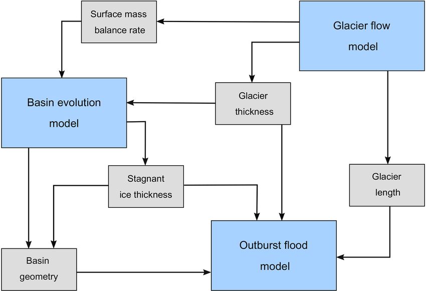
336                                           A. Jenson et al.: Long-period variability in ice-dammed glacier outburst floods

Figure 2. Model schematic illustrating the glacier and basin geometry (for a wedge-shaped basin).

energy requires that                                                      The basin is assumed to be completely filled with ice at
                                                                     year 0, at which point the tributary glacier detaches from the
                 ∂N                                                    trunk glacier and leaves behind remnant ice. Initially the rem-
ṁLf = Q ψ +           .                                      (4)
                 ∂s                                                    nant ice may be attached to the trunk glacier and act like a
                                                                       floating ice tongue, but ultimately it breaks into a pack of ice-
Two boundary conditions are required to solve this system of           bergs. We assume that the remnant ice thins at a rate given by
equations. We set the effective pressure at the terminus equal         the specific surface mass balance rate. Thus, we neglect re-
to 0. At the basin outlet, the effective pressure is                   plenishment of ice into the basin via glacier flow or iceberg
                                                                       calving. We further assume that the remnant ice is sufficiently
Nb = ρi gHb − (ρw ghw + ρi ghi ),                             (5)
                                                                       mobile and fractured to form a horizontal layer of thickness
                                                                       hi as the basin fills. We therefore assume that drainage pro-
where Hb and hw are the glacier thickness and water depth at
                                                                       ceeds quickly enough that the floating ice thickness does not
the basin outlet and hi is the thickness of floating ice in the
                                                                       change during the course of the outburst flood and conse-
basin. Variations in water level are related to the basin hyp-
                                                                       quently ice is stranded on the basin walls (see Fig. 2). The
sometry and discharge into and out of the basin, as described
                                                                       floating ice volume at time t is given by
in Sect. 2.1.2 (see Eq. 10). In addition, the ice dam height
and floating ice thickness both vary during glacier recession                        Zt
(Sect. 2.2).                                                           Vi = Vi,0 +        Ḃb Ab (Hb ) dt 0 ,                       (7)
2.1.2   Basin hypsometry and evolution                                               t0

We assume that the ice-dammed basin has an idealized hyp-              where subscript “, 0” refers to initial conditions, Ḃb is the
sometry that can be described by                                       specific surface mass balance rate (see Sect. 2.2) at the
                                                                       basin’s elevation, and we apply the mass balance rate to the
             p−1                                                       surface of the remnant ice.
Ab (zb ) = azb     ,                                          (6)
                                                                         The volume of water stored in the basin Vw for a given
where Ab is the mapview area of the basin at different el-             water depth is
evations, zb is the elevation relative to the lowest point in                 a p
the basin, and a and p are constants that describe the basin           Vw =     hw .                                                (8)
                                                                              p
shape. For reference, p = 1, p = 2, and p = 3 describe box-,
wedge-, and semicircular-cone-shaped basins, respectively.             Since a and p are constants for a given basin, the water vol-
We define Wb , Lb , and θb as the basin width, length, and             ume in the basin can be expressed as
bed slope (Fig. 2). For a box-shaped basin a = Wb Lb , for
                                                                                hw p

a wedge-shaped basin a = Wb cot θb , and for a semicircular-
cone-shaped basin a = (π/2)cot2 θb .                                   Vw =            Vw,0 .                                    (9)
                                                                               hw,0

The Cryosphere, 16, 333–347, 2022                                                                https://doi.org/10.5194/tc-16-333-2022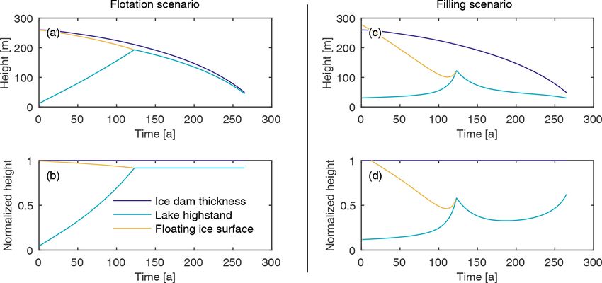
A. Jenson et al.: Long-period variability in ice-dammed glacier outburst floods                                                           337

Table 1. List of model parameters. Values of constants are specified in brackets.

                       Variable          Description
                       ρi , ρw           densities of ice [917 kg m−3 ] and water [1000 kg m−3 ]
                       g                 gravitational acceleration [9.81 m s−2 ]
                       Lf                latent heat of fusion [3.34 × 10⁵ J kg−1 ]
                       A, n              ice flow law parameter [2.4 × 10⁻²⁴ Pa−3 s−1 ] and exponent [3]
                       K                 ice flow parameter for conduit closure [1.78 × 10⁻²⁵ Pa−3 s−1 ]
                       f , n0            friction factor [0.066 m−2/3 s2 ] and hydraulic roughness [0.1 m1/3 ]
                       x, s, z, zb       horizontal, bed-parallel, and vertical coordinates and elevation relative to ice dam base
                       θ, L, S, ṁ       conduit slope, length, cross-sectional area, and melt rate
                       Q, Qin , Qb       discharge along the conduit, discharge into the basin, and discharge from the basin
                       M                 water flux to the conduit per unit length
                       Pi , N, ψ         ice-overburden pressure, effective pressure, and basic hydraulic gradient
                       hw , hi           basin water depth and floating ice thickness
                       S0 , hw,0         initial cross sectional area and initial basin water depth
                       Hb , Nb           ice dam thickness and effective pressure
                       Ab                mapview area of the basin
                       a, p              coefficient and exponent that describe basin hypsometry
                       Wb , Lb , θb      basin width, length, and bed slope
                       Vi , Vw           volumes of ice and water in the basin
                       Vs                basin storage capacity (volume of water when basin is at flotation depth)
                       H , hs , W , U    glacier thickness, surface elevation, width, and depth- and width-averaged velocity
                       Ub , Uc           ice velocity toward the basin and calving rate into the basin
                       τ , τmax          basal shear stress and maximum basal shear stress [2.5 × 10⁵ Pa]
                       ν                 ice viscosity
                       Ḃ, Ḃmax , Ḃb   width-averaged, maximum, and basin specific mass balance rates
                       ELA               equilibrium line altitude

The volume fluxes of water entering and leaving the basin                      Since the ice volume is known (Eq. 7), hi (and therefore hw,0 )
are Qin and Qb . Thus, we find the rate of change of the wa-                   can be determined by adjusting its value until Eqs. (7) and
ter surface elevation by setting the time derivative of Eq. (9)                (12) are in agreement. In the second scenario (“filling sce-
equal to Qin − Qb and rearranging, which yields                                nario”) we set the initial water level to hw,0 = 10 m and the
                  p                                                            discharge into the lake to Qin = 20 m3 s−1 , which allows the
dhw     hw,0                                                                   basin to fill while draining. In both scenarios, we assume
    =   p−1
               (Qin − Qb ).                                          (10)
 dt   phw Vw,0                                                                 the filling rate Qin remains constant despite the changing
                                                                               climate and year-to-year variability. We tested values of 0–
We consider two scenarios for evolving the water level. In                     25 m3 s−1 , and while different values of Qin impact the flood
the first scenario (“flotation scenario”) we assume that the                   magnitudes and how quickly a flood is initiated, we found
effective pressure is initially zero at the basin outlet and that              that varying Qin does not qualitatively affect our results, and
the basin begins to drain shortly after starting each simula-                  so we chose to keep Qin constant throughout the filling sce-
tion. In this scenario we set Qin = 0 m3 s−1 since the basin                   nario simulations. Additionally, Qin has little impact on the
is already full and the flood occurs soon after the simulation                 outburst flood hydrographs once a flood initiates because the
begins. The initial water level is                                             flood discharge exceeds Qin by more than 2 orders of mag-
           ρi                                                                  nitude. Note that we only apply the filling scenario to box-
hw,0 =        (Hb − hi ),                                            (11)
           ρw                                                                  shaped basins in order to avoid geometric complexities asso-
                                                                               ciated with raising and lowering a fragmented layer of rem-
and the volume of floating ice is related to its thickness by
                                                                               nant ice along a sloping basin, and therefore we compute the
integrating Eq. (6) and substituting in Eq. (11):
                                                                               floating ice thickness by simply dividing the ice volume by
       hi Z
          +hw,0                                                                the basin surface area. We define basin storage capacity, Vs ,
Vi =           azb
                      p−1
                            dzb                                                as the water volume when the basin level is at flotation depth
                                                                               and the peak water volume as the volume of water when the
       hw,0
                             p               p                           lake in a simulation has reached peak water depth. In the
       a          ρi                ρi                                         flotation scenario, basin storage capacity and peak water vol-
   =         hi +    (Hb − hi ) −      (Hb − hi )     . (12)
       p          ρw                ρw

https://doi.org/10.5194/tc-16-333-2022                                                                    The Cryosphere, 16, 333–347, 2022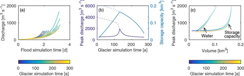
338 A. Jenson et al.: Long-period variability in ice-dammed glacier outburst floods
ume are equal; however, in the filling scenario, the peak water where ν is the depth- and width-averaged viscosity, U is the
volume is less than the basin storage capacity for all simula- depth- and width-averaged velocity, W is glacier width, τ is
tions. the basal shear stress, and hs is the glacier surface elevation.
The viscosity depends on the strain rate according to Glen’s
2.1.3 Numerics flow law:
2/3
The outburst flood model is nondimensionalized and solved ∂U
ν = A−1/3 . (14)
numerically using methods described by Kingslake (2013) ∂x
and Kingslake and Ng (2013a). We use a constant time step
in dimensionless units, resulting in the dimensional time step We assume a simplified ad hoc parameterization of the basal
decreasing from ∼ 400 to ∼ 300 s as the glacier thins and re- shear stress, in which τ = τmax (U/max(U )), with τmax =
treats. For the grid spacing we set ds = s/100, which equals 2.5 × 10⁵ Pa. This parameterization results in shear stresses
∼ 50 m at year 0 and decreases as the glacier retreats. At each on the order of 105 Pa, which are typical values for valley
time step, given S, hw , and hi , we solve Eqs. (2) and (3) si- glaciers (e.g., Brædstrup et al., 2016), and produces realis-
multaneously for N and Q, with m defined by Eq. (4), dS/dt tic glacier geometries and velocities across a wide range of
in Eq. (2) provided by Eq. (1), and the boundary condition bed slopes and climates. Importantly, the parameterization
on N at the lake provided by Eq. (5). Employing an approach ensures that the resistive stresses never exceed the glaciolog-
referred to as the relaxation method by Kingslake (2013), a ical driving stress. For boundary conditions, we prescribe a
fictitious time derivative is introduced to the left of Eq. (2), velocity of U = 0 at the ice divide (x = 0) and velocity gra-
and, after making an initial guess at the discharge at the lake dient ∂U/∂x = 0 at the terminus (x = L).
Q0 , the result is solved with Eq. (3) using the forward Euler The glacier surface is updated using a depth- and width-
method in time and an upwind difference in space until the integrated mass continuity equation (van der Veen, 2013), in
fictitious derivative disappears. This is performed repeatedly which
within a root-finding algorithm, which tunes Q0 , until the N ∂H 1 ∂(U H W )
boundary condition (Eq. 5) is met. This results in profiles of = Ḃ − , (15)
∂t W ∂x
N and Q that obey Eqs. (2) and (3) and the boundary con-
ditions. These are used to evolve hw and S forward in time where Ḃ is the width-averaged specific mass balance rate.
with Eqs. (10) and (1), respectively. Initial values for hw and We prescribe the mass balance rate by using a constant mass
S are discussed in Sect. 2.3. balance gradient and imposing a maximum balance rate Ḃmax
(as is commonly observed; e.g., Van Beusekom et al., 2010).
2.2 Glacier evolution In other words,
We model changes in glacier geometry with a one- dḂ
Ḃ(z) = min (z − ELA), Ḃmax , (16)
dimensional form of the shallow shelf approximation (SSA), dz
which is a depth- and width-integrated flow model (Nick
where ELA is the equilibrium line altitude. We use an initial
et al., 2009; Enderlin et al., 2013; Carnahan et al., 2019). For
ELA of 1500 m, a balance gradient of dḂ/dz = 0.005 a−1 ,
our simulations, we use a glacier with a simple bed geometry
and a maximum balance rate of Ḃmax = 2 m a−1 . The ELA
(a uniformly sloping bed with a slope of 4◦ ) and assume a
increases at a rate of 5 m a−1 to approximate expected
simple climate parameterization. After running the model to
changes under climate warming scenarios (Huss and Hock,
steady state, we invoke glacier retreat by applying a constant
2015).
rate of warming. The simulations are run until the glacier ter-
The model equations are discretized following the
minus retreats past the basin, which is initially located 75 %
methodology described in Enderlin et al. (2013) using finite
of the way from the head of the glacier to its terminus. We
differences for the spatial discretization (initial grid spacing
ran additional simulations with different parameter values
of 100 m); a staggered, moving grid; and a forward Euler
for bed slope, climate, and basin location. Although these
time step (1t = 0.05 a). At each time step, Eq. (13) is solved
parameters affect the details of how outburst floods change
for the velocity, and the glacier surface is adjusted according
from year to year, they do not affect the overall pattern of
to Eq. (15). The glacier length is updated by allowing the ter-
how floods evolve.
minus to advance at its flow speed, and any ice thinner than
The glacier flow model is based on conservation of mo-
0.1 m is subsequently removed from the domain.
mentum, which requires that the glaciological driving stress
is balanced by gradients in longitudinal stress, lateral drag, 2.3 Simulations
and basal drag (van der Veen, 2013), such that
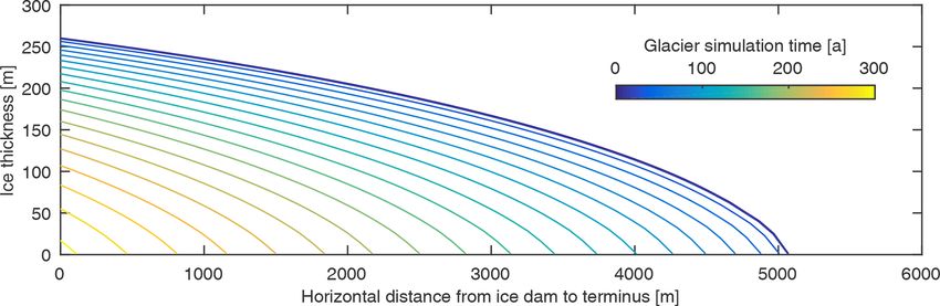
In the glacier flow model it takes about 300 years for the
5U 1/3
∂ ∂U H ∂hs glacier terminus to retreat from its initial position to the lo-
2 Hν − − τ = ρi gH , (13) cation of the marginal basin, a distance of ∼ 5 km (Fig. 3).
∂x ∂x W 2AW ∂x
The Cryosphere, 16, 333–347, 2022 https://doi.org/10.5194/tc-16-333-2022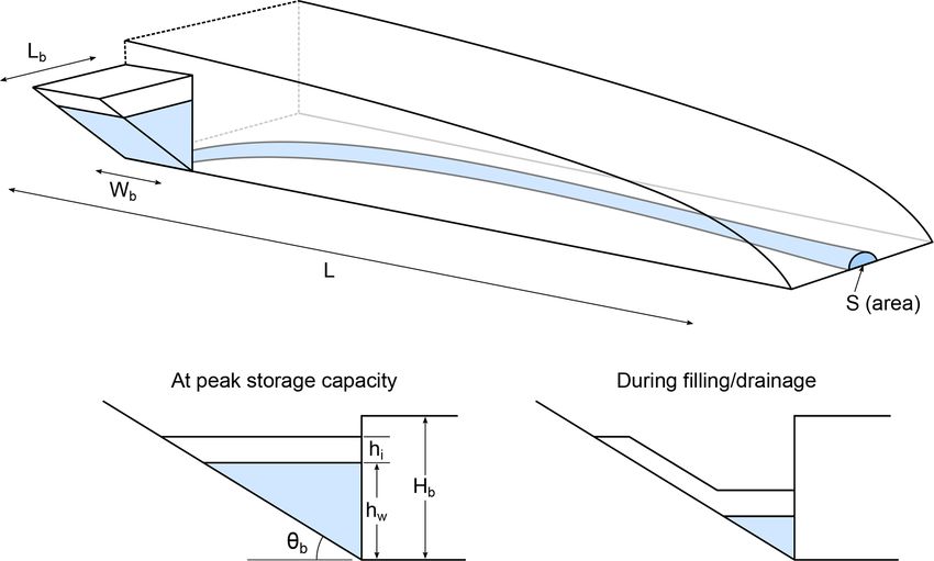
A. Jenson et al.: Long-period variability in ice-dammed glacier outburst floods                                                       339

Figure 3. Ice thickness profile from the marginal basin to the terminus over 300 years of glacier retreat.

For each year of the glacier model output, we extract (i) the             of its behavior during filling and drainage nontrivial. The
distance from the basin to the terminus, which we take to                 floating ice should gradually expand outward as the basin
equal the conduit length; (ii) the glacier thickness profile and          fills, but then friction should prevent it from flowing back
ice dam thickness; and (iii) the specific mass balance rate of            down to the bottom of the basin during rapid drainage. In
the ice dam. Then (i) and (ii) are fed directly into the out-             the filling scenario the basin generally does not fill up com-
burst flood model, and (iii) is used to calculate the volume of           pletely, greatly complicating the task of tracking the thick-
floating ice remaining in the basin (Fig. 4).                             ness and location of the floating ice except when the basin
   To demonstrate how remnant ice affects outburst floods,                walls are vertical. For this reason we only apply the filling
we first run simulations in which we use the glacier geom-                scenario to box-shaped basins.
etry from one time step in the glacier flow model, assume a
box-shaped basin, and run the outburst flood model with dif-
ferent starting water volumes. We run the simulations both                3   Results
without ice and with enough ice to force ice dam flotation.
Thus, these initial simulations are similar to those that we              For glaciers with a fixed geometry, floating ice in a basin
run in the flotation scenario (next paragraph) except that here           causes outburst floods to have higher peak discharge and
the basin is not necessarily at flotation depth unless it con-            shorter duration than might otherwise be expected based
tains remnant ice.                                                        solely on the consideration of flood water volume (Fig. 6).
   We then use the evolving glacier and basin geometries                  Consequently, changes in remnant ice volume impact the
to model long-period variations in outburst floods using the              evolution of glacier outburst floods over decadal to centen-
flotation and filling scenarios described in Sect. 2.1.2. In the          nial timescales. In our transient glacier simulations we ob-
flotation scenario, we assume that the initial water pressure             served similar trends in flood hydrographs regardless of basin
at the basin outlet equals the overburden pressure of the ice             hypsometry and whether the simulations started with the
dam. In this scenario, the initial conduit area is 1 m2 . Thus,           basins filled to flotation depth (Fig. 7) or if the basins were
we assume that the basin is not connected to the subglacial               connected to the subglacial hydrological system as they filled
drainage system until the onset of the outburst flood. To test            (Fig. 8). The floods that occur in the years immediately fol-
the effect of basin geometry and floating ice on outburst flood           lowing the formation of a marginal basin have low peak dis-
evolution, we run simulations with (i) box-shaped, wedge-                 charge on account of the basin’s small storage capacity. As
shaped, and semicircular-cone-shaped basins and (ii) both                 the climate warms, the remnant ice thins more quickly than
with and without floating ice (Fig. 5). For the box-shaped                the ice dam, which is partially replenished by the delivery of
basin we used a value of a = 8.5 × 10⁵ m2 , for the wedge-                ice from upstream. The largest outburst floods occur when
shaped basin we used a basin width of 1910 m and a bed                    the basin becomes ice-free, after which the peak discharge
slope of 15◦ , and for the semicircular-cone-shaped basin we              decreases until the basin is no longer dammed by the trunk
used a bed slope of 10.6◦ . These values were chosen so that              glacier.
the basins would initially have the same basin storage capac-                For the simulations in which the basins were filled to flota-
ity Vs .                                                                  tion depth before flood onset, we considered three different
   In the filling scenario we prescribe a small initial water             basin hypsometries (semicircular-cone-, wedge-, and box-
level of 10 m and an initial conduit area of 0.1 m2 . The sub-            shaped) that had identical storage capacities at the time of
glacial conduit is connected to the marginal basin as filling             basin formation (year 0). The cone-shaped basin produced
occurs, and the conduit therefore evolves prior to the onset              the largest outburst floods in terms of peak discharge, how-
of the outburst flood, which occurs naturally once Qb > Qin .             ever flood magnitude decreased more rapidly across the sim-
The granular nature of the floating ice makes a full treatment            ulations for the cone-shaped basin compared to the wedge-
                                                                          and box-shaped basins (Fig. 7a–c). The differences in peak

https://doi.org/10.5194/tc-16-333-2022                                                              The Cryosphere, 16, 333–347, 2022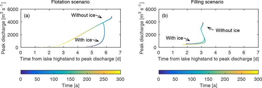
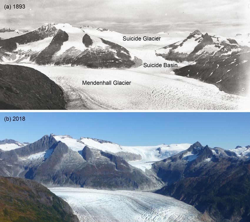
340                                              A. Jenson et al.: Long-period variability in ice-dammed glacier outburst floods

Figure 4. Information flow between the glacier flow, basin evolution, and outburst flood models.

Figure 5. Schematic of the various scenarios that we considered in our simulations, illustrating basin geometry, presence/absence of remnant
ice, and whether drainage initiated when the lake reached flotation depth or while the basin was filling. For the flotation scenario, we prescribe
Qin = 0 m3 s−1 , S0 = 1 m2 , and hw,0 = (Hb − hi )ρi /ρw (flotation depth). For the filling scenario simulations, we prescribe the discharge
into the basin as Qin = 20 m3 s−1 , the initial conduit cross-sectional area as S0 = 0.1 m2 , and the initial water level hw,0 = 10 m. The basins
all have the same initial volume (year 0 in the ice flow model), but as the ice dam thins the changes in basin volume are nonlinear for the
cone- and wedge-shaped basins. The simulations with remnant ice assume the basin is completely filled with ice at year 0.

discharge and duration of large magnitude floods arise be-                 discharge and peak water volume (which is often less than
cause, owing to their hypsometry, cone-shaped basins lose                  the storage capacity, as defined above) takes a slightly dif-
their floating ice more rapidly than wedge- or box-shaped                  ferent form. First, the basin often does not reach flotation
basins and because as they drain the floating ice in the basin             depth in our simulations because the conduit enlarges at the
exerts pressure on the underlying water that helps to drive                same time as the basin is filling and consequently the outburst
the water out of the basin. However, ice-dam thinning re-                  floods tend to be smaller in magnitude (Fig. 8). This behav-
duces basin capacity faster in cone-shaped basins than in                  ior is sensitive to the model parameters though, as the basin
wedge- or box-shaped basins, and therefore the magnitude                   could be made to reach or even exceed flotation depth by se-
of the outburst floods in cone-shaped basins decreases more                lecting a larger influx Qin . Second, there is a more prominent
rapidly. In the early years of the simulations, flood magni-               spike in the peak discharge curve that occurs as the remnant
tude increases in basins that are initially filled with ice (solid         ice is about to melt away completely (Fig. 8b). Similar to the
line) until the basin is ice-free, whereas in basins that are              flotation scenario, the relationship between peak discharge
initially ice-free (dotted line) the flood magnitude always de-            and peak water volume is approximately linear; however, in
creases (Fig. 7d–f). For all three hypsometries we observe a               the filling scenario the peak water volume is less than the
nearly linear relationship between peak discharge and stor-                storage capacity because the basin does not completely fill
age capacity (Fig. 7g–i). This relationship holds regardless               (Fig. 8c). As a result the relationship between peak discharge
of whether the basin contains ice or is ice-free.                          and (total) storage capacity is not linear.
   For the simulations in which the basin is initially drained                Figures 7 and 8 show that remnant ice can act to pro-
of water but remains connected to the subglacial hydrolog-                 duce similar size outburst floods for very different glacier
ical system as the basin fills, the relationship between peak              thicknesses. To further illustrate this consequence of remnant

The Cryosphere, 16, 333–347, 2022                                                                  https://doi.org/10.5194/tc-16-333-2022
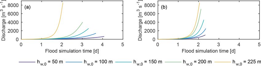
A. Jenson et al.: Long-period variability in ice-dammed glacier outburst floods                                                               341

Figure 6. Demonstration of the impact of floating ice on outburst flood hydrographs for an ice dam height of 250 m (year 50 in the glacier
simulations). The glacier geometry and basin shape (box) are the same in all simulations. In panel (a), the initial water height, hw,0 , is varied
and there is no floating ice in the basin. The initial water heights are the same in panel (b) except that enough floating ice is added to force
ice dam flotation. For hw,0 = 225 m, the water level is equal to flotation depth so there is no remnant ice, and the curves in panels (a) and
(b) are the same. Note that the modeled hydrographs do not include the rapidly falling limb of the floods because the outburst flood model is
not capable of handling open channel flow, which occurs when the basin water level drops below the conduit roof.

Figure 7. Comparison of annual outburst floods for semicircular-cone-, wedge-, and box-shaped basins for the simulations in which the basin
is initially at flotation depth. (a–c) Annual outburst flood hydrographs when the basin is initially filled with ice. (d–f) Peak discharge and
storage capacity over time. The fork in the early years of the simulations represents ice-filled (solid line) and ice-free (dotted line) scenarios.
(g–i) Peak discharge vs. storage capacity for the ice-filled scenario. We refer to the timescale of the glacier flow model as “glacier simulation
time” and the timescale of the outburst flood model as “flood simulation time”.

ice, we plot peak discharge versus ice dam height for the                   210 m). On the other hand, when remnant ice is excluded
box-shaped basin in both the filling and flotation scenarios                from the simulations, the peak discharge increases monoton-
(Fig. 9). In the flotation scenario we observe large variabil-              ically with ice dam height in both the flotation and filling
ity in outburst floods during glacier recession; for example,               scenarios. Thus, proper accounting of remnant ice is critical
a peak discharge of 2000 m3 s−1 occurs when the ice dam                     for quantifying the evolution of outburst floods over decadal
height is 240 m and then again when it is 120 m. In contrast,               to centennial timescales.
in the filling scenario, the peak discharge is nearly indepen-
dent of ice dam height except during the years in which the
basin becomes ice-free (when the ice dam height was around

https://doi.org/10.5194/tc-16-333-2022                                                                 The Cryosphere, 16, 333–347, 2022
342 A. Jenson et al.: Long-period variability in ice-dammed glacier outburst floods
Figure 8. Comparison of annual outburst floods for the box-shaped basin in which the basin is connected to the subglacial hydrological
system as it fills. (a) Annual outburst flood hydrographs. (b) Peak discharge and basin storage capacity for ice-filled and ice-free basins. The
fork in the early years of the simulations represents ice-filled (solid line) and ice-free (dotted line) scenarios. (c) Relationship between peak
discharge and peak water volume (“Water”) and basin storage capacity (“Storage capacity”).
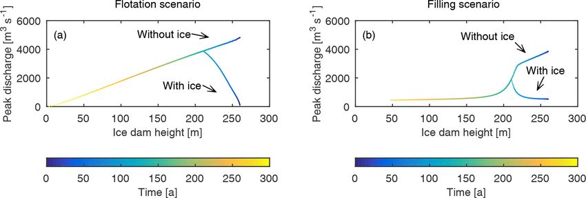
Figure 9. Comparison of peak discharge and ice dam height for the box-shaped basin under the (a) flotation scenario and (b) filling scenarios.
“With ice” indicates the relationship between peak discharge and ice dam height when remnant ice is accounted for in the model, whereas
“Without ice” indicates the relationship when remnant ice is neglected.
4 Discussion Taking the derivative of Eq. (17) with respect to time, we find
that storage capacity evolves according to
4.1 Impact of remnant ice and ice flow on basin storage " p−1 #
dVs ρi dHb dhi
capacity = a (Hb − hi ) − . (18)
dt ρw dt dt
During decadal- to centennial-scale glacier retreat, the peak The term in square brackets in Eq. (18) is always positive,
discharge of ice-dammed outburst floods will tend to increase and thus the storage capacity will always increase as long as
with time as long as there is remnant ice in a basin that dHb /dt > dhi /dt (i.e., the ice dam is thinning less quickly
is melting away. The peak discharge will begin to decrease than the remnant ice). Thinning of the ice dam due to sur-
only once the remnant ice is gone. This result is indepen- face melting is partially offset by ice flow from upglacier,
dent of basin geometry and the mechanism of drainage onset and therefore the storage capacity, and by extension the peak
and is ultimately a consequence of the proportionality be- discharge of outburst floods, will continue to increase until a
tween peak discharge and basin storage capacity that occurs basin is ice-free.
for individual basins despite large changes in glacier geome- However, in our simulations we did not account for ice
try and remnant ice. In other words, the model exhibits very flow or calving of icebergs into a basin, which would require
little hysteresis between peak discharge and basin storage ca- a significantly more sophisticated ice flow model. Ice flow
pacity (Figs. 7g–i and 8c). As a result, the time rate change into a basin shortens the basin and reduces the storage ca-
of the basin storage capacity illuminates how peak discharge pacity. Calving changes the basin geometry but tends to have
evolves with time. The storage capacity is found by inserting little net impact on storage capacity because it has two com-
Eq. (11) into Eq. (8), which gives peting effects: it results in retreat of an ice dam away from
a basin, which increases storage capacity, but it also adds to
the volume of remnant ice, which reduces storage capacity.
p
a ρi For a more detailed discussion on the impacts of ice flow and
Vs = (Hb − hi ) . (17) calving on storage capacity, see Appendix A.
p ρw
The Cryosphere, 16, 333–347, 2022 https://doi.org/10.5194/tc-16-333-2022A. Jenson et al.: Long-period variability in ice-dammed glacier outburst floods 343
Our analysis here has focused solely on basin storage ca- with time, or are ice-free. We also find that the slopes of the
pacity. The relationship between peak discharge and water discharge-volume curves depend on basin geometry, where
volume is likely to become more complicated than presented basins that contain less volume near their outlets produce
in Figs. 7 and 8 when changes in basin geometry due to ice a steeper slope. This is likely a result of cone- and wedge-
flow and calving are accounted for. Moreover, we do not ac- shaped basins being able to maintain high water pressures as
count for lateral variations in glacier thickness that may cause they drain, thus favoring more rapid conduit growth.
the seal of the ice dam to be located some distance from the The explanation for the lower, 2/3 exponent in the
basin. Flow redirection toward a marginal basin due to lateral Clague–Mathews relationship remains elusive. Ng and
surface gradients will affect the ice dam thinning rates and lo- Björnsson (2003) suggest that the lower exponent is due to
cation of the seal in ways that we are unable to capture in our differences in flood initiation across different basins (im-
one-dimensional flowline model. These additional complex- plying that flood initiation may depend on basin hypsome-
ities should be considered in more detail in future studies. try). Flood initiation could also depend on some time-varying
property such as ice dam thickness or the size of a previous
4.2 Comparison to the Clague–Mathews relationship year’s flood, both of which could influence the state of the
subglacial hydrological system at the onset of a flood (see
Observations across a range of systems are suggestive of a also Kingslake, 2015). For example, some flood events in-
power-law relationship between the peak discharge and total volving large volumes of water (i.e., when the basin stor-
water volume drained, 1Vw , during outburst floods (Clague age capacity is large) have a persistent impact on the sub-
and Mathews, 1973; Walder and Costa, 1996): glacial system, so that when a basin refills it does so while
Qpeak ∝ 1Vw 2/3 . (19) slowly draining, whereas floods involving small volumes of
water may have a less persistent impact, and as a result subse-
This relationship is commonly referred to as the Clague– quent floods will only initiate after the basin reaches flotation
Mathews relationship. Ng and Björnsson (2003) examined depth.
the Clague–Mathews relationship by analyzing the equa-
tions describing flood evolution. Using a simplified version 4.3 Hazard assessment confounded by poor
of the outburst flood model used in this study, they demon- understanding of drainage onset
strated that for individual basins that do not drain completely,
(i) each flood trajectory has a unique set of initial and final Mitigating risks due to outburst floods requires accurate pre-
water levels and peak discharge, (ii) peak discharge mono- dictions of flood initiation, peak discharge, and flood dura-
tonically increases with water volume, and (iii) there is a tion. As our results show, these properties depend on basin
power-law relationship between discharge and water volume hypsometry and the amount of remnant ice in a basin, which
for floods. They focused on analyzing basins that experi- may be unknown in many situations, making it difficult to
ence incomplete drainage because some information on flood assess current and future outburst flood hazards. In contrast,
mechanics is lost if a basin drains completely. Their anal- changes in ice dam thickness are much easier to observe,
ysis predicts an exponent in the power-law relationship of making it tempting to try to relate ice dam thickness to poten-
about 1–2 for individual basins, depending on basin geom- tial flood magnitudes. However, our simulations (Figs. 7 and
etry and ice coverage. When observed flood data from mul- 8) suggest that similar size outburst floods may occur for very
tiple glaciers were scaled and placed into their theoretical different ice dam thicknesses if a basin contains remnant,
framework, they arrived at an exponent close to 1. They hy- floating ice. This nonlinearity occurs both for basins that do
pothesized that the difference between their theoretical expo- not connect to the hydrological system until drainage onset
nent and the exponent in the Clague–Mathews relationship is (flotation scenario) and for basins that remain connected to
due to confounding factors such as differences in flood initi- the subglacial hydrological system during filling (filling sce-
ation, basin geometry, and complete drainage. nario) (Fig. 9).
Our simulations extend the work of Ng and Björns- Remnant, floating ice affects outburst floods in multiple
son (2003). We modeled variations in outburst floods over ways that also affect hazard assessment. First, the presence of
decadal to centennial timescales, from different shaped floating ice reduces the storage capacity of a basin (Figs. 7d–f
basins, and with different drainage scenarios (flotation vs. and 8b). Shortly after a basin forms, the presence of remnant
filling). In addition, in our simulations the basins always ice limits the storage capacity and causes the peak discharge
drained completely. We observe that the relationship between to be small. As the ice melts over time the storage capacity
peak discharge and peak water volume reached (equal to vol- and peak discharge increase until the basin is ice-free. The re-
ume drained) is nearly linear in the flotation scenario (power- lationship is more clearly seen in the flotation scenario than
law exponent of ∼ 1; Fig. 7g–i) and superlinear in the fill- in the filling scenario (Fig. 10). Floods tend to be more uni-
ing scenario (power-law exponent > 1; Fig. 8c). These trends form from year to year in the filling scenario because when
occur regardless of whether the basins contain remnant ice, floating ice is present, the additional pressure causes the out-
in which case peak discharge and storage capacity increase let conduit to open relatively quickly, and the basin drains
https://doi.org/10.5194/tc-16-333-2022 The Cryosphere, 16, 333–347, 2022344 A. Jenson et al.: Long-period variability in ice-dammed glacier outburst floods
Figure 10. Time series of the ice dam elevation, lake highstand (peak water surface), and floating ice surface elevation at lake highstand for
the (a) flotation and (b) filling scenarios. In panels (c) and (d), the values for height are normalized using the ice dam thickness as a measure
of scale.
before filling to flotation depth. Further, once the floating Kienholz et al., 2020) and is also likely related to the onset
ice has melted and the ice dam is thinner, the ice-overburden mechanism. A deeper understanding of the onset of outburst
pressure is less and the creep closure is slowed down by the floods is therefore critical to improving our ability to assess
increasing water pressure as the basin is filling. As a result, both the short- and long-term risk associated with outburst
melt opening overcomes creep closure, which acts to initiate floods.
a flood more quickly, and again the basin only fills partially
(Fig. 10c–d).
A second consequence of floating ice is that it affects the 5 Conclusions
duration of outburst floods (Fig. 11). The role of floating ice
We modeled the effect of changes in glacier and basin ge-
is again most clear in the flotation scenario. Early in the sim-
ometries on the magnitude and duration of ice-dammed
ulations, when the storage capacity is small, outburst floods
glacier outburst floods. In our simulations we accounted for
that have higher peak discharge than might be expected can
remnant, floating ice that is left behind in marginal basins
occur because the pressure from the floating ice helps to drive
during the retreat of tributary glaciers. The remnant ice exerts
water out of the basin. However, the small amounts of water
pressure on the underlying water and thus helps to increase
(relative to the size of the basin) in these events are not able
discharge by enlarging the subglacial conduit. Because the
to melt the conduit walls as rapidly as later floods, and the
remnant ice is not replenished by ice flow from upglacier,
overburden pressure from the ice dam, which favors creep
it thins more quickly than the adjacent ice dam. As a re-
closure, is high. Consequently, the floods tend to be slower
sult the basin storage capacity increases with time as long
building and the basins may take about a week to drain. Later,
as the basin contains remnant ice, regardless of basin hyp-
when the floating ice is gone and the ice dam is also thinner,
sometry. Despite complex relationships between glacier and
drainage can proceed more quickly. This creates challenges
basin hypsometry, remnant ice thickness, and discharge, we
for flood risk mitigation because floods with similar peak dis-
find nearly linear relationships between peak outburst flood
charges may occur over timescales of a few days (e.g., An-
discharge and total water volume for individual basins. This
derson et al., 2003) to a week (e.g., Huss et al., 2007) de-
is regardless of whether the basin drains once it reaches flota-
pending on basin conditions (Fig. 11a). For basins that fill
tion depth or if it remains connected to the subglacial hydro-
while connected to the subglacial hydrological system, there
logical system while filling. However, differences in modeled
tends to be less variability in the duration of outburst floods
outburst floods for the two different drainage scenarios that
(Fig. 11b).
we considered highlight the importance of improving our un-
Our simulations predict differences in how outburst floods
derstanding of drainage onset. Basins that are continuously
will evolve with time, depending on whether a basin begins
connected to the subglacial drainage system tend to produce
to drain once it has filled or if the basin remains connected to
similar outburst floods from one year to the next, except dur-
the subglacial hydrological system and begins to drain as it
ing the years immediately before and after the loss of rem-
is filling. Furthermore, our model does not address the large
nant ice, whereas basins that do not begin to drain until full
year-to-year variability in peak discharge and total water vol-
produce much larger variability in the magnitude and timing
ume of outburst floods, which may vary by a factor of 2 or
of outburst floods.
more in subsequent years (e.g., Huss et al., 2007; Neal, 2007;
The Cryosphere, 16, 333–347, 2022 https://doi.org/10.5194/tc-16-333-2022A. Jenson et al.: Long-period variability in ice-dammed glacier outburst floods 345
Figure 11. Comparison of peak discharge and time from lake highstand to peak discharge for the box-shaped basin under the (a) flotation
and (b) filling scenarios.
In our simulations we made a number of simplifying as- the ice dam. The rate of change of the storage capacity is
sumptions in order to garner a fundamental understanding of
the long-period variability of outburst floods in an evolving dVs ρi dHb dhi
= − Wb Lb
catchment. In particular, we (1) assumed that the seal of the dt ρw dt dt
ice dam was immediately adjacent to the basin and did not ρi dLb
account for changes in the hydraulic potential gradient that + (Hb − hi ) Wb . (A2)
ρw dt
could drive water from the glacier into the basin as it is fill-
ing; (2) treated remnant ice as a fluid that spreads out as a The thickness of the remnant ice changes at a rate that is
basin fills, instead of accounting for the granular nature of given by
the icebergs; (3) did not consider the state of the glacier’s hy-
dhi Hb hi dLb
drological system at the time of drainage, which may impact = Ḃb + Uc − , (A3)
flood evolution, or changes in ice flow due to the evolving dt Lb Lb dt
subglacial hydrology; (4) did not allow for ice flow into the where Uc is the calving rate. The three terms on the right-
basin from the trunk glacier; and (5) did not account for inter- hand side of Eq. (A3) describe the changes in ice thickness
annual variability in climate and its effects on glacier geome- due to the surface mass balance, the influx of freshly calved
try and basin filling rates. Year-to-year variability in the tim- ice, and changes in the ice dam location. The rate of change
ing, duration, and magnitude of outburst floods (e.g., Huss of the basin length is simply dLb /dt = Uc − Ub , where Ub is
et al., 2007; Neal, 2007; Kienholz et al., 2020) may mask the the rate at which ice is flowing toward the basin. By inserting
longer period changes in outburst floods due to changes in these expressions for dhi /dt and dLb /dt into Eq. (A2) and
glacier and basin geometry that we modeled here. Additional rearranging, we find that
and more sophisticated modeling studies will be needed to
elucidate the impact of these processes on the decadal and 1 ρw dVs dHb
= Lb − Ḃb Lb − Ub Hb , (A4)
centennial evolution of outburst floods and to connect out- Wb ρi dt dt
burst floods to landscape and ecosystem evolution.
which indicates that the storage capacity will increase as long
as dHb /dt > Ḃb + Ub Hb /Lb . For a box-shaped basin the ef-
fects of calving cancel out completely, and changes in storage
Appendix A: Effect of ice flow and calving on basin capacity are only due to thinning of the ice dam, the surface
storage capacity of a box-shaped basin mass balance rate, and the ice flux toward the basin. The ef-
fect of ice flow is to reduce the maximum storage capacity
that occurs in a basin and to increase the time that it takes
For a box-shaped basin, the basin storage capacity is given
for the maximum storage capacity to be reached since con-
by
traction of the remnant ice reduces the surface area that is
susceptible to melting.
ρi
Vs = (Hb − hi )Wb Lb . (A1) Equation (A4) illustrates that ice flow toward a basin may
ρw have important consequences for basin storage capacity. For
example, the remnant ice in Suicide Basin, the source of
Since we are now allowing for ice flow and calving, the basin recent outburst floods at Mendenhall Glacier, has a surface
length is no longer treated as a constant and the remnant ice mass balance flux (Ḃb Lb Wb ) of about −2.5 × 10⁶ m3 a−1 ,
thickness varies in response to the addition of new icebergs and the ice flux toward the basin (Ub Hb Wb ) is roughly 3.5–
and compaction/extension due to changes in the location of 7.0×10⁵ m3 a−1 (both expressed as ice equivalent) (Kienholz
https://doi.org/10.5194/tc-16-333-2022 The Cryosphere, 16, 333–347, 2022346 A. Jenson et al.: Long-period variability in ice-dammed glacier outburst floods
et al., 2020); thus, ice flow is currently offsetting the growth Brædstrup, C. F., Egholm, D. L., Ugelvig, S. V., and Pedersen, V.
in storage capacity due to melting by about 25 %. K.: Basal shear stress under alpine glaciers: insights from ex-
periments using the iSOSIA and Elmer/Ice models, Earth Surf.
Dynam., 4, 159–174, https://doi.org/10.5194/esurf-4-159-2016,
Code availability. MATLAB script files for the full model 2016.
are available at https://doi.org/10.5281/zenodo.5488047 (Jenson, Capps, D. M., Rabus, B., Clague, J. J., and Shugar, D. H.: Identi-
2021). fication and characterization of alpine subglacial lakes using in-
terferometric synthetic aperture radar (InSAR): Brady Glacier,
Alaska, USA, J. Glaciol., 56, 861–870, 2010.
Carnahan, E., Amundson, J. M., and Hood, E.: Impact of glacier
Data availability. No data sets were used in this article.
loss and vegetation succession on annual basin runoff, Hydrol.
Earth Syst. Sci., 23, 1667–1681, https://doi.org/10.5194/hess-23-
1667-2019, 2019.
Author contributions. JMA and EH conceived the study, AJ ran the Carrivick, J. L. and Tweed, F. S.: A review of glacier
simulations with assistance from JMA and JK, and AJ and JMA outburst floods in Iceland and Greenland with a
prepared the manuscript with contributions from JK and EH. megafloods perspective, Earth Sci. Rev., 196, 102876,
https://doi.org/10.1016/j.earscirev.2019.102876, 2019.
Clague, J. J. and Mathews, W. H.: The Magnitude of jökulhlaups, J.
Competing interests. The contact author has declared that neither Glaciol., 12, 501–504, 1973.
they nor their co-authors have any competing interests. Clague, J. J., Huggel, C., Korup, O., and Mcguire, B.: Cli-
mate Change and Hazardous Processes in High Mountains,
Revista de la Asociacion Geologica Argentina, 69, 328–338,
Disclaimer. Publisher’s note: Copernicus Publications remains https://doi.org/10.5167/uzh-77920, 2012.
neutral with regard to jurisdictional claims in published maps and Cook, K. L., Andermann, C., Gimbert, F., Adhikari, B. R.,
institutional affiliations. and Hovius, N.: Glacial lake outburst floods as drivers
of fluvial erosion in the Himalaya, Science, 362, 53–57,
https://doi.org/10.1126/science.aat4981, 2018.
Acknowledgements. This project was supported by funding from Cuffey, K. M. and Paterson, W. S. B.: The physics of glaciers, Else-
the Alaska Climate Adaptation Science Center and the US National vier, Amsterdam, 4 edn., 2010.
Science Foundation (OIA-1757348 and OPP-1743310). We thank Enderlin, E. M., Howat, I. M., and Vieli, A.: High sensitivity of
Christian Kienholz for fruitful discussions that led to this study. tidewater outlet glacier dynamics to shape, The Cryosphere, 7,
1007–1015, https://doi.org/10.5194/tc-7-1007-2013, 2013.
Evatt, G. W.: Röthlisberger channels with finite ice
Financial support. This research has been supported by the Alaska depth and open channel flow, J. Glaciol., 56, 45–50,
Climate Adaptation Science Center, University of Alaska Fairbanks https://doi.org/10.3189/2015AoG70A992, 2015.
(Alaska NSF EPSCoR, grant no. OIA-1208927), and the National Flowers, G., Bjornsson, H., Palsson, F., and Clarke, G.: A coupled
Science Foundation (grant no. OPP-1743310). sheet-conduit mechanism for jokulhlaup propagation, Geophys.
Res. Lett., 31, L05401, https://doi.org/10.1029/2003GL019088,
2004.
Fowler, A. C.: Breaking the seal at Grimsvötn, Iceland, J. Glaciol.,
Review statement. This paper was edited by Johannes J. Fürst and
45, 506–516, https://doi.org/10.3189/S0022143000001362,
reviewed by two anonymous referees.
1999.
Huss, M. and Hock, R.: A new model for global glacier
change and sea-level rise, Front. Earth Sci., 3, 54,
https://doi.org/10.3389/feart.2015.00054, 2015.
References Huss, M. and Hock, R.: Global-scale hydrological response to
future glacier mass loss, Nat. Clim. Change, 8, 135–140,
Anderson, S. P., Walder, J., Anderson, R., Kraal, E., Cunico, https://doi.org/10.1038/s41558-017-0049-x, 2018.
M., Fountain, A., and Trabant, D.: Integrated hydrologic and Huss, M., Bauder, A., Werder, M., Funk, M., and
hydrochemical observations of Hidden Creek Lake jökulh- Hock, R.: Glacier-dammed lake outburst events of
laups, Kennicott Glacier, Alaska, J. Geophys. Res., 108, 6003, Gornersee, Switzerland, J. Glaciol., 53, 189–200,
https://doi.org/10.1029/2002JF000004, 2003. https://doi.org/10.3189/172756507782202784, 2007.
Bigelow, D. G., Flowers, G. E., Schoof, C. G., Mingo, L. D. B., Jenson, A. J.: amyjenson/glacier-basin-outburst-flood-model:
Young, E. M., and Connal, B. G.: The role of englacial hydrology glacier-basin-outburst flood model (subglacial_hydrology),
in the filling and draining of an ice-dammed lake, Kaskawulsh Zenodo [code], https://doi.org/10.5281/zenodo.5488047, 2021.
Glacier, Yukon, Canada, J. Geophys. Res.-Earth Surf., 125, Keisling, B. A., Nielsen, L. T., Hvidberg, C. S., Nuterman, R., and
e2019JF005110, https://doi.org/10.1029/2019JF005110, 2020. DeConto, R. M.: Pliocene–Pleistocene megafloods as a mecha-
Bjornsson, H.: Jokulhlaups in Iceland: prediction, char- nism for Greenlandic megacanyon formation, Geology, 48, 737–
acteristics and simulation, Ann. Glaciol., 16, 95–106, 741, https://doi.org/10.1130/G47253.1, 2020.
https://doi.org/10.3189/1992AoG16-1-95-106, 1992.
The Cryosphere, 16, 333–347, 2022 https://doi.org/10.5194/tc-16-333-2022You can also read