Reconstructing winter climate anomalies in the Euro-Atlantic sector using circulation patterns
←
→
Page content transcription
If your browser does not render page correctly, please read the page content below

Weather Clim. Dynam., 2, 777–794, 2021
https://doi.org/10.5194/wcd-2-777-2021
© Author(s) 2021. This work is distributed under
the Creative Commons Attribution 4.0 License.

Reconstructing winter climate anomalies in the
Euro-Atlantic sector using circulation patterns
Erica Madonna1 , David S. Battisti2 , Camille Li1 , and Rachel H. White3
1 Geophysical Institute, University of Bergen and Bjerknes Centre for Climate Research, Bergen, Norway
2 Department of Atmospheric Sciences, University of Washington, Seattle, WA, USA
3 Department of Earth, Ocean and Atmospheric Sciences, University of British Columbia, Vancouver, BC, Canada

Correspondence: Erica Madonna (erica.madonna@uib.no)

Received: 25 January 2021 – Discussion started: 28 January 2021
Revised: 11 June 2021 – Accepted: 29 June 2021 – Published: 25 August 2021

Abstract. The efficacy of Euro-Atlantic circulation regimes        2016). The seasonal climate signal results from a succession
for estimating wintertime climate anomalies (precipitation         of daily weather that is often organized by the large-scale
and surface temperature) over Europe is assessed. A com-           flow into a finite number of preferred circulation patterns,
parison of seasonal climate reconstructions from two dif-          also called regimes (Corte-Real et al., 1995; Molteni et al.,
ferent regime frameworks (cluster analysis of the low-level        1990; Vautard, 1990). Therefore, one might expect that sea-
zonal flow, and traditional blocking indices) is presented         sonal climate anomalies could be reconstructed from the fre-
and contrasted with seasonal reconstructions using the North       quency of the dominant atmospheric patterns over a season.
Atlantic Oscillation (NAO) index. The reconstructions are          This approach has been used to study future trends in Eu-
quantitatively evaluated using correlations and the coefficient    ropean precipitation (Santos et al., 2016) and as a predictor
of efficiency, accounting for misfit in phase and amplitude.       for droughts (Lavaysse et al., 2018). It can also be used to
The skill of the various classifications in reconstructing sea-    better understand and anticipate the changes in weather pat-
sonal anomalies depends on the variable and region of inter-       terns that sum to the seasonal to decadal climate anomalies
est. The jet and blocking regimes are found to capture more        that stem from predictable changes in the atmosphere–ocean
spatial structure in seasonal precipitation anomalies over Eu-     system, such as those associated with the El Niño–Southern
rope than the NAO, with the jet framework showing gen-             Oscillation phenomenon and the Atlantic multidecadal vari-
erally better skill relative to the blocking indices. The re-      ability associated with the ocean overturning circulation in
constructions of temperature anomalies have lower skill than       the North Atlantic (see Battisti et al., 2019, for a review).
those for precipitation, with the best results for temperature        Atmospheric variability patterns can be characterized in
obtained by the NAO for high-latitude and by the blocking          several ways, such as by the North Atlantic Oscillation in-
framework for southern Europe. All methods underestimate           dex (NAO, e.g. Hurrell, 1995), the occurrence of blocking
the magnitude of seasonal anomalies due to the large vari-         (e.g. Pfahl and Wernli, 2012; Sillmann and Croci-Maspoli,
ability in precipitation and temperature within each classifi-     2009; Trigo et al., 2004), and the configuration of the North
cation pattern.                                                    Atlantic jet stream (Woollings et al., 2010; Madonna et al.,
                                                                   2017). All these complementary classifications have been
                                                                   shown to be able to capture specific aspects of the winter-
                                                                   time climate over Europe, but there has been to our knowl-
1   Introduction                                                   edge no direct comparison of the skill of these classifications
                                                                   in reconstructing seasonal climate.
Seasonal precipitation and temperature anomalies over Eu-             In this study we compare how well European winter con-
rope exhibit large year-to-year variability, with direct soci-     ditions are described by indices of the NAO, blocking, and
etal impacts such as on crop yields and renewable energy           North Atlantic jet configurations. The NAO manifests as sea
production (Grams et al., 2017; Jerez et al., 2013; Lesk et al.,

Published by Copernicus Publications on behalf of the European Geosciences Union.
778                                                E. Madonna et al.: Reconstructing winter climate using circulation patterns

                                                                       (Woollings et al., 2010; Davini et al., 2014; Madonna et al.,
                                                                       2017).
                                                                          These classifications of North Atlantic atmospheric vari-
                                                                       ability thus offer closely related but alternative views of sea-
                                                                       sonal climate fluctuations. For example, an extreme season
                                                                       may occur due to the unusual persistence or frequency of a
                                                                       certain jet configuration (Madonna et al., 2019), without a
                                                                       corresponding extreme value of the NAO index or blocking
                                                                       pattern. This study aims to compare the ability of three clas-
                                                                       sification methods (NAO, blocking, jet configurations) to re-
                                                                       construct seasonal climate anomalies over Europe. By know-
                                                                       ing the frequency of each circulation pattern, we assess the
                                                                       skill of each method to reproduce the sign (i.e. correlation)
                                                                       and amplitude (i.e. ratio of standard deviations) of seasonal
Figure 1. Winter (DJF) blocking climatology (shading, as % of          precipitation and temperature anomalies.
time). The green and black boxes show the domain used for the def-
inition of the NAO and jet clusters, respectively. The orange, blue,
and red boxes denote the regions used for Greenland blocking (GB),
                                                                       2     Methods and data
Iberian wave breaking (IWB), and Scandinavian Blocking (SBL),
respectively.
                                                                       We focus on the low-level wind (900 to 700 hPa), 2 m tem-
                                                                       perature (T2m), and total precipitation. The analyses are
                                                                       conducted for winter (DJF; the 90 d period 1 December–
                                                                       28 February), with ERA-Interim reanalysis (Dee et al., 2011)
level pressure (SLP) fluctuations with anticorrelated extrema          for the period 1979–2014, interpolated to a 0.5◦ horizontal
between two poles: one over the Azores and one over Iceland.           resolution. To identify blocking, 6-hourly data of geopoten-
These fluctuations signify changes in the prevailing westerly          tial height at 500 hPa are used. For the rest of the analysis,
winds and in the propagation path of storms into Europe (e.g.          daily means are used.
Hurrell, 1995; Hurrell et al., 2003; Qian et al., 2000; Rogers,
                                                                       2.1     Classifications
1997; Wanner et al., 2001). In contrast, blocking is the pres-
ence of a persistent and stationary high-pressure system that          2.1.1    NAO
obstructs or deviates the westerly flow (Rex, 1950). In the
North Atlantic sector blocking occurs mainly over three re-            We use the daily NAO time series from NOAA (down-
gions: Greenland, Scandinavia, and the Iberian Peninsula               loaded from ftp://ftp.cpc.ncep.noaa.gov/cwlinks/norm.daily.
(Treidl et al., 1981; Davini et al., 2014, also shown in Fig. 1).      nao.index.b500101.current.ascii, last access: 14 May 2020),
Precipitation is reduced within the blocked region (Sousa              which is calculated using geopotential height at 500 hPa and
et al., 2017) while cold temperature extremes are often ob-            covers the whole North Atlantic basin north of 20◦ N (green
served southeast of the blocked region (Sillmann and Croci-            box in Fig. 1). A day is classified as a positive (negative)
Maspoli, 2009). Lastly, jet configurations describe preferred          NAO day if its NAO value is above 0.5 (below −0.5) of
flow paths of the North Atlantic jet stream, which acts as             the wintertime NAO standard deviation. The remaining days,
waveguide for midlatitude storms (Athanasiadis et al., 2010;           about 35 d per winter (Table 1), are considered neutral NAO
Hoskins and Ambrizzi, 1993; Wettstein and Wallace, 2010;               days.
Wirth et al., 2018). In winter the North Atlantic jet stream
can assume five different configurations (southern, central,           2.1.2    Blocking
northern, tilted, and mixed, Madonna et al., 2017) with dis-
tinct patterns of storm propagation, all of which are associ-          Blocking events are identified on 6-hourly data following the
ated with regional climate anomalies over Europe.                      criteria from Scherrer et al. (2006), which define a block as a
   The three classification methods for circulation regimes            reversal in the meridional gradient of the geopotential height
that we use in this study are not independent: the strength            at 500 hPa in a 30◦ latitudinal band that lasts for at least 5 d.
and position of the jet are intrinsically linked to changes in         Climatologically in the North Atlantic there are three main
SLP and thus to the NAO and blocking; blocking over Green-             regions affected by blocking (shading in Fig. 1): one over
land, Scandinavia, and the Iberian Peninsula correspond to a           Greenland, one over northern Europe/Scandinavia, and one
southern, mixed, and northern configuration of the jet stream,         offshore of the Iberian Peninsula. Note that the enhanced fre-
respectively (Madonna et al., 2017). However, the NAO does             quency at 30◦ N is an artefact of the detection method (see
not map clearly onto distinct jet configurations or blocking           discussion in Davini et al., 2014). We define three boxes to
patterns, with the positive phase being especially ambiguous           capture these three regions: Greenland (65–25◦ W, 60–75◦ N,

Weather Clim. Dynam., 2, 777–794, 2021                                                      https://doi.org/10.5194/wcd-2-777-2021
E. Madonna et al.: Reconstructing winter climate using circulation patterns                                                                  779

Table 1. Average and (in brackets) standard deviation of the num-            the central jet resembles the zonal/NAO+ regime, the mixed
ber of days per winter in each category. The positive (negative) NAO         jet resembles the Scandinavian blocking regime, and the
phase is defined as days with NAO values above 0.5 (below −0.5)              southern jet resembles the Greenland anticyclone/NAO−
of the time series standard deviation (see Sect. 2 for more infor-           regime (see Fig. 8 in Madonna et al., 2017). Using five clus-
mation), and the remaining days are considered as neutral. We dif-           ters, the zonal regime can be further separated into a central
ferentiate between blocking over Greenland (GB), over the Iberian
                                                                             and tilted jet (see Fig. 10 in Madonna et al., 2017). In this
Peninsula (IWB), Scandinavia (SBL) and non-blocked days (NB).
The categories for the jet are south (S-jet), tilt (T-jet), north (N-jet),
                                                                             study, we use five jet clusters, which gives more distinct jet
mixed (M-jet), and central (C-jet). We also reported the number of           configurations over the North Atlantic.
days in the undefined category using the jet classification (undef).            We calculate the daily mass-weighted average zonal wind
                                                                             (U ) between 900–700 hPa in the sector 60◦ W–0◦ , 15–75◦ N
           NAO                   Blocking                  Jet               (black box, Fig. 1) and use this field to calculate jet clusters
                                                                             as described in Madonna et al. (2017). We perform an EOF
 NAO−        25.4 (16.8)   GB       13.5 (11.4)    S-jet      7.3 (7.7)
 NAO+        30.0 (13.9)                           T-jet     12.0 (9.8)
                                                                             analysis on the low-level wind to reduce the dimensions and
                           IWB      13.0 (12.3)    N-jet      8.6 (7.5)      apply a k-means clustering algorithm to the first five principal
                           SBL       16.9 (9.3)    M-jet      9.7 (7.4)      components, which explains up to 80 % of the wintertime
                                                   C-jet    10.9 (11.0)      variability in that sector.
 neutral     34.6 (11.1)   NB       51.9 (14.0)    undef    41.4 (10.0)         Every day is associated with a cluster depending on the
                                                                             normalized inverse Euclidean distance (d) from the cluster
                                                                             centroid (i.e. d = 1 at the centroid location and d = 0 far
                                                                             from the centroid) in the five-dimensional space of the prin-
GB, orange box in Fig. 1), Scandinavia (15◦ W–25◦ E, 50–                     cipal components. The Euclidean distance (E) from the cen-
65◦ N, SBL, red box), and offshore of the Iberian Penin-                     troid c forq a point x in a n-dimensional space is defined as
sula (30◦ W–0◦ , 40–50◦ N, named as in Davini et al. (2014)                                 Pn               2
                                                                             E(c, x) =         i=1 (ci − xi ) . E is normalized such that the
Iberian wave breaking (IWB), blue box).
                                                                             proximity measure d = 1/E sums to 1 over all days. Since
   A day is considered a blocked day if at least 10 % of the
                                                                             some days can be close to more than one centroid, in partic-
grid points in the respective box satisfy the blocking criteria.
                                                                             ular during transition days from one cluster to the other, we
This choice reduces the number of blocking events identi-
                                                                             keep only days whose d to the respective centroid is larger
fied as it detects blocking episodes at a later stage of their
                                                                             than 0.5. A sensitivity analysis suggests that the choice of
development (i.e. when they are spatially larger) than if no
                                                                             the threshold d does not have a significant impact on the
threshold were applied, and avoids the detection of blocks
                                                                             results (see Supplement). Approximately 54 % of the 3150
that are predominantly located upstream or downstream of
                                                                             (= 35×90) d are unequivocally attributed to a specific cluster
the boxed regions. Table 1 reports the average (standard de-
                                                                             (see Table 1, 41.4 d, i.e. 46 % are not assigned to any cluster).
viation) number of days per winter with blocking at different
                                                                                The five clusters represent a southern jet (S-jet), a cen-
locations. During the 35 winters, we detect on average 13.5 d
                                                                             tral jet (C-jet), a northern jet (N-jet), a tilted jet (T-jet), and a
per winter of GB, 16.9 of SBL, and 13.0 of IWB while 51.9 d
                                                                             mixed jet (M-jet with a split structure). On average each clus-
are considered as “non blocked” (NB). It can occasionally
                                                                             ter occurs between 7.3 d (S-jet) and 12.0 d (T-jet) per winter,
happen that during a single day several regions are simul-
                                                                             as reported in Table 1, with large winter-to-winter variability
taneously blocked. Therefore, the sum of blocking and NB
                                                                             (standard deviation).
days does not sum to exactly 90 d (i.e. one winter).

2.1.3      Jet clusters                                                      2.1.4   Associated weather anomalies

Cluster analysis applied to SLP or geopotential height is                    Each NAO phase, blocking category, and jet cluster is char-
commonly used to classify circulation patterns into so-called                acterized by different circulation, precipitation, and temper-
weather regimes. In the North Atlantic during winter, four                   ature anomalies. We compute daily anomalies of zonal wind,
classical regimes are identified (e.g Cassou, 2008; Michelan-                precipitation, and temperature and then construct compos-
geli et al., 1995; Vautard, 1990), although the optimal num-                 ites for each NAO phase, blocking category, and jet cluster
ber of clusters is not clear-cut and depends somewhat on the                 by averaging the daily fields of all (defined) days belong-
algorithm, atmospheric field, domain, and considered tem-                    ing to the corresponding category. For wind and precipita-
poral period (Christiansen, 2007; Dorrington and Strommen,                   tion the daily anomalies are calculated by subtracting the cli-
2020; Falkena et al., 2020; Woollings et al., 2010). Madonna                 matological 35-year winter mean, as previous studies have
et al. (2017) showed that applying a cluster analysis to the                 shown a weak seasonal cycle of those variables within DJF
low-level jet leads to four jet configurations that correspond               (Woollings et al., 2014; Zveryaev, 2004). However, the sea-
to the four classical weather regimes in the Euro-Atlantic                   sonal cycle is much stronger for temperature and therefore
sector: the northern jet resembles the Atlantic Ridge regime,                temperature anomalies are calculated by removing the daily

https://doi.org/10.5194/wcd-2-777-2021                                                          Weather Clim. Dynam., 2, 777–794, 2021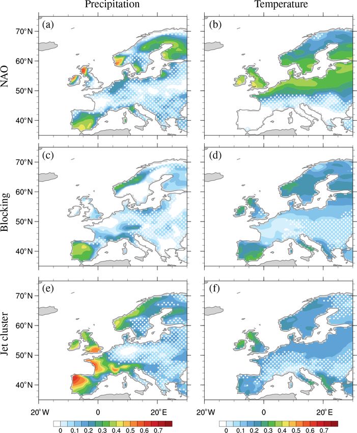
780                                                              E. Madonna et al.: Reconstructing winter climate using circulation patterns

35-year average, smoothed with a 30 d running mean. The
                                                                                                    (ot − pt )2
                                                                                                     P
resulting anomalies are presented in Sect. 3.1.
                                                                                                         t
                                                                                          CE ≡ 1 − P            ,                                                (3)
2.2     Seasonal reconstructions                                                                     (ot − o)2
                                                                                                             t
To reconstruct the seasonal anomalies we count the number
of days in each NAO phase, blocking category, and jet cluster                             where ( ) denotes the mean of a quantity and the sum is over
for each winter. Similar to Cortesi et al. (2019), we then re-                            all winter seasons (t).
construct the seasonal precipitation and temperature anomaly                                 Equation (3) can be rewritten as
maps Arec (φ, λ, t) for each season (t) as follows:                                                  σ 2 (o0 ) + σ 2 (p 0 ) − 2 < o0 , p 0 > /N + (o − p)2
                                                                                          CE ≡ 1 −                                                           ,   (4)
                                                                                                                        σ 2 (o0 ) + o2
                 X
Arec (φ, λ, t) =    (Yi (φ, λ) · fi (t)),                  (1)
                        i
                                                                                          where (0 ) denotes the anomaly about the mean ( ) and σ is
where φ, λ, and t are latitude, longitude, and time, respec-                              the standard deviation.
tively; i represents the two NAO phases, three blocking cat-                                 If we consider only anomalies and therefore assume that
egories, or five jet clusters; Yi (φ, λ) are the maps of seasonal                         the mean of o and p are both zero, the equation can be sim-
average precipitation/temperature anomalies associated with                               plified such that
the considered pattern; fi (t) is the fraction of time the pattern
                                                #days of pattern i
occurs in the given season t (i.e. fi (t) = #days  per season (=90) ).
                                                                                          CE ≡ 2ra − a 2 ,                                                       (5)
   For example for the jet clusters in DJF 2013/14 (cf. Fig. 5),
there are 0 d classified as S-jet and M-jet, 11 d as T-jet, 7 d                           where a is an amplitude ratio of the standard deviations of
as N-jet, and 60 d as C-jet. The remaining 12 d belong to                                 the time series,
the undefined category and are not used. The reconstructed                                     σ (p)
anomaly using the jet clusters for DJF 2013/14 is                                         a=         ,                                                           (6)
                                                                                               σ (o)
Arec (φ, λ, 2013/14) =
0 · YS (φ, λ) + 0 · YM (φ, λ) + 11 · YT (φ, λ) + 7 · YN (φ, λ) + 60 · YC (φ, λ)
                                                                                          and r is the correlation between o and p.
                                                                                ,   (2)      In our case, o is the observed anomaly of precipita-
                                      90
                                                                                          tion/temperature and o is by definition zero, while p is the
where the Yi (φ, λ) are the composite maps of precipitation                               reconstructed anomaly and p is not necessarily zero (see
or temperature anomalies, and the subscript stands for the jet                            Fig. S2). In this study, the CE is calculated using Eq. (3),
type.                                                                                     while the simplification (Eq. 5) is used for scaling the
   This reconstruction method assumes that the average of                                 anomaly amplitudes (see Sect. 3.3).
the undefined days represents the climatological mean; i.e.                                  When applied to reconstructions and observations, the CE
the average anomaly field associated with undefined days is                               is a measure of skill in reconstruction that is more restric-
close to zero. In the Supplement (Fig. S1) we show that this                              tive than a simple correlation because it penalizes for both
is indeed the case. In the case of the residual not summing                               phase and amplitude misfits. For a perfect reconstruction,
to zero, Eq. (1) must be modified to include the pattern and                              CE = 1. For a reconstruction with observed variance (a = 1)
the fraction of time of the unclassified days. To compare the                             that is correlated with the observed time series of seasonal
ability of each classification method to reconstruct seasonal                             anomalies at r = 0.5, the result is CE = 0. For a reconstruc-
anomalies, we compute at each grid point the correlation as                               tion that is perfectly correlated with observations but with
well as the coefficient of efficiency (CE, described in the next                          twice the observed amplitude, we arrive at the same result
section) between the reconstructed and the observed (ERA-                                 of CE = 0. We consider CE > 0.25 to indicate a good recon-
Interim) seasonal anomalies.                                                              struction. A reconstruction that has perfect variance (a = 1)
                                                                                          and CE = 0.25 would explain 39 % of the observed variance
2.2.1     Coefficient of efficiency (CE)
                                                                                          (r = 0.63); given 35 years of data (degrees of freedom), this
Assume o is the observed quantity and p is the reconstructed                              correlation would be significant at p = 0.0001. For a recon-
quantity. The coefficient of efficiency (CE) (Nash and Sut-                               struction with perfect correlation (i.e. r = 1), CE > 0.25 can
cliffe, 1970; see also Bürger, 2007; Briffa et al., 1992; Wang                            be obtained for amplitude values 0.13 < a < 1.87. As the CE
et al., 2014), which we calculate at each grid point (φ, λ), is                           maximizes when r = a (and max(CE) = r 2 ), a CE of 0.25
given by                                                                                  also implies a minimum correlation of 0.5 independent of the
                                                                                          amplitude error. For this reason, only points with correlation
                                                                                          greater than 0.5 are considered when optimizing the CE (see
                                                                                          Sect. 3.3).

Weather Clim. Dynam., 2, 777–794, 2021                                                                           https://doi.org/10.5194/wcd-2-777-2021
E. Madonna et al.: Reconstructing winter climate using circulation patterns                                                          781

Figure 2. Zonal wind anomalies (shading, in m s−1 ) at 850 hPa for two NAO phases (first column), three blocking categories (second
column), and five jet clusters (third column). Black contours show the climatological zonal wind at 850 hPa (contours at 5 and 10 m s−1 ).
The figure is organized such that maps in the same row represent similar circulation patterns identified by more than one method (NAO,
blocking, jet regime).

3     Results                                                          show precipitation and temperature anomalies (colours), re-
                                                                       spectively, and the composite zonal wind (black contours).
3.1    Classification of anomalies and interannual                     The panels are arranged such that each row includes “sim-
       variability                                                     ilar” (based on temporal correlation shown in Fig. 5) pat-
                                                                       terns identified using the NAO index (left column), block-
Distinct wind, temperature, and precipitation anomalies are            ing (centre column), and the jet clusters (right column). In
associated with each NAO phase, blocking category, and jet             general, wind and temperature patterns along each row are
cluster (Figs. 2–4). Figure 2 shows the zonal wind anoma-              remarkably similar given the composites including different
lies for each pattern (colours) and the climatological DJF             numbers of days; e.g. for the top row, there are on average
zonal wind distribution (black contours). Figures 3 and 4              25.4 d per season corresponding to the NAO− group, 13.5 d

https://doi.org/10.5194/wcd-2-777-2021                                                    Weather Clim. Dynam., 2, 777–794, 2021
782                                              E. Madonna et al.: Reconstructing winter climate using circulation patterns

to GB, and 7.3 d to S-jet (see Table 1). Despite similarity in          The zonal wind anomaly composites of the days that are
the spatial structures of the composites, there can be large         not included in any category are close to zero for the NAO
differences in the strength of the anomalies for the different       (neutral days) and for the jet (undefined), but not for the non-
classification methods.                                              blocked (NB) category (see Fig. S1). This behaviour can be
   The top rows of Figs. 2–4 show a clear correspon-                 understood from the point of view of the classical weather
dence between the negative NAO phase, Greenland blocking             regimes, as the non-blocked category includes days that be-
(GB), and the S-jet cluster, consistent with previous work           long to the “zonal/NAO+” regime as well as days with weak
(Woollings et al., 2010; Madonna et al., 2017). In all three         wind anomalies. Therefore, in terms of zonal wind, the com-
composites the jet is located southwards of its climatological       posite of non-blocked days is very different from climatol-
position (Fig. 2). This southerly shifted jet is also zonally ori-   ogy. However, this effect is less evident in the precipitation
ented, which can be seen in the total composite wind fields          and temperature anomalies (i.e. anomalies close to zero).
shown in black contours in Figs. 3 and 4. In all three com-             The correspondence between the jet and blocking compos-
posites, precipitation is enhanced in the jet core and at its        ites extends to seasonal timescales. Figure 5 shows the time
ends, e.g. over the Iberian Peninsula (Fig. 3, blue shading).        series of the occurrence (i.e. the number of days per win-
Although the patterns look fairly similar, they differ in inten-     ter) of each NAO phase, blocking, and jet cluster. The time
sity, with the highest precipitation anomalies found in the S-       series of the S-jet cluster has a correlation of 0.64 with GB
jet cluster. When the jet is shifted south (NAO−, GB, S-jet),        and 0.67 with the negative NAO phase. However, the S-jet is
Greenland is warmer than usual, while northern Europe and            less frequent than the other two, with on average only 7.3 d
the Barents Sea are colder than usual (Fig. 4, shading). The         per winter, compared to 13.5 d of GB and 25.4 d of the nega-
anomaly patterns shown in the top row resemble the Green-            tive NAO phase (Table 1). The N-jet occurs on average 8.6 d
land anticyclone/NAO− regime in the framework of the four            per winter and IWB 13.0 d (Table 1), and their time series
classical Euro-Atlantic weather regimes (e.g. cf. with Catti-        (Fig. 5b) are correlated at 0.71. The M-jet occurs on average
aux et al., 2013; van der Wiel et al., 2019).                        9.7 d, SBL 16.9 d, and their time series are correlated at 0.58.
   There is less correspondence between the positive NAO             The C-jet (10.9 d) and T-jet (12.0 d) are the most frequent jet
phase and any other pattern. As the positive NAO phase has           clusters; however, they show a relatively low correlation with
often been referred to as the unblocked or unperturbed state         the positive NAO time series (0.30 and 0.45, respectively).
(e.g. Woollings et al., 2008, 2010), it does not resemble any           The winter to winter differences in the number of days
of the blocking patterns. The positive NAO composite has             in each jet cluster and blocking type is large: standard de-
wind and temperature anomaly patterns reminiscent of both            viations are of similar magnitude to the mean values (Ta-
the tilted and central jet clusters (Figs. 2 and 4, shadings),       ble 1). Moreover, about 40 %–60 % of the days are classi-
with a jet shifted to the north (and tilted) and warmer temper-      fied as NAO neutral days, unblocked, or undefined (for the
atures over central and northern Europe. The warm anomaly            jet cluster). The composites of precipitation and temperature
over the Barents Sea observed during the positive NAO phase          for those categories are similar to climatology, and therefore
is weakly present in both the tilted and central jet composites,     their patterns are characterized by little anomalies, in partic-
while the cold anomaly over Greenland is linked to the tilted        ular over the European continent (Fig. S1).
jet rather than the central jet. Also, precipitation anomalies of
the positive NAO phase are more similar to the tilted jet clus-      3.2     Seasonal reconstructions
ter than the central jet cluster, indicative of the large change
in precipitation pattern associated with the relatively small        Using the method described in Sect. 2.2, we reconstruct sea-
shifts in jet position.                                              sonal anomalies of temperature and precipitation from each
   Blocking over the Iberian Peninsula (IWB) is associated           of the three classification methods: the NAO, blocking, and
with a northward shift of the jet (N-jet), while blocking over       jet clusters. Based on our definitions, for each classifica-
Scandinavia (SBL) splits the jet, resulting in a M-jet con-          tion the average number of days per season used for recon-
figuration (Madonna et al., 2017). Translated into the four          struction is between 38.1 d (blocking composites) and 55.4 d
classical weather regimes, blocking in these regions thus oc-        (NAO composites; Table 1). We compare our reconstructed
curs during the Atlantic Ridge and Scandinavian blocking             seasonal anomalies to the observed anomalies to evaluate the
regimes, respectively (Madonna et al., 2017). The blocked            skill of each method for precipitation and temperature.
region is drier than climatology for both cases (Fig. 3), with
less precipitation offshore and over the Iberian Peninsula as-       3.2.1    Correlation
sociated with the N-jet cluster (IWB), and less precipita-
tion over central Europe associated with the M-jet cluster           The ability of each method to reconstruct seasonal weather
(SBL). During IWB, southern Europe and northern Africa               anomalies varies greatly with location. To assess this, we
are colder, while northern Europe is warmer than normal;             calculate for each grid point the correlation coefficient be-
during N-jet, only the cold anomaly is evident. During SBL,          tween the time series of seasonal reconstructed anomalies
most of Europe is cold and northern Scandinavia is warm.             and that of the actual anomalies from the ERA-Interim re-

Weather Clim. Dynam., 2, 777–794, 2021                                                   https://doi.org/10.5194/wcd-2-777-2021

E. Madonna et al.: Reconstructing winter climate using circulation patterns                                                       783

Figure 3. Precipitation anomalies (shading, in mm d−1 ) and zonal wind at 850 hPa (contours at 5, 10, and 15 m s−1 ) for two NAO phases
(first column), three blocking categories (second column), and five jet clusters (third column).

analysis. Figure 6 shows the spatial distribution of this cor-        culation than does temperature, as temperature can be af-
relation coefficient over Europe for precipitation (Fig. 6a, c        fected by other mechanisms including cloud cover and land
and e) and temperature (Fig. 6b, d and f); regions are masked         surface feedbacks. The correlation coefficients for wind are
with white dots when the correlation coefficient is below 0.5.        much higher than those of precipitation and temperature for
The spatial structure of correlations for temperature is much         all classifications (Fig. S3).
smoother than that for precipitation; this is consistent with            Overall, the correlations between precipitation reconstruc-
smoother variations in temperature fields relative to precipi-        tions and observations are higher in western Europe and
tation, which varies at much smaller spatial scales. For the re-      Scandinavia and lower in central to south-east Europe. Re-
constructions based on jet clusters, precipitation agrees bet-        gions with low correlations also show little seasonal variabil-
ter (higher correlations) with observations than temperature,         ity (i.e. small seasonal standard deviations, Fig. S4) suggest-
in particular in regions of high topography. In these regions         ing that large-scale circulation patterns have less impact on
it is likely that precipitation depends more uniquely on cir-         precipitation in these regions. There are relatively minor dif-

https://doi.org/10.5194/wcd-2-777-2021                                                  Weather Clim. Dynam., 2, 777–794, 2021
784                                             E. Madonna et al.: Reconstructing winter climate using circulation patterns

Figure 4. Two-metre temperature anomalies (T2m, shading, in ◦ C) and zonal wind at 850 hPa (black contours at 5, 10, and 15 m s−1 ) for
two NAO phases (first column), three blocking categories (second column), and five jet clusters (third column).

ferences in the correlation of precipitation for the different        variability exhibits a southwest–northeast gradient (Fig. S4),
methods, although correlations over France are noticeably             and regions with larger variability (e.g. Scandinavia) often
worse in the NAO reconstruction (cf. Fig. 6a with c and e).           exhibit larger correlations for all classification methods.
   The skill of the temperature reconstructions depends
greatly on the classification method. Over Spain and France,          3.2.2   Coefficient of efficiency
the blocking method does substantially better than the NAO
and slightly better than the jet clusters. Conversely, the NAO        Having shown strong correlations between reconstructed and
performs much better in a band from 50 to 65◦ N than the              observed seasonal anomalies for many regions of Europe, we
other methods but substantially worse south of 50◦ N. This is         now examine the coefficient of efficiency (CE), which takes
consistent with the temperature anomalies in Fig. 4 – neither         into account both the correlation (i.e. the phase) and the mag-
positive nor negative NAO is associated with strong temper-           nitude of the reconstructed values relative to observations.
ature anomalies across southern Europe. Winter temperature            The spatial pattern of the CE for precipitation (Fig. 7) gener-

Weather Clim. Dynam., 2, 777–794, 2021                                                    https://doi.org/10.5194/wcd-2-777-2021

E. Madonna et al.: Reconstructing winter climate using circulation patterns                                                             785

Figure 5. Time series of the number of days per winter for different categories: (a) negative NAO phase (NAO−), Greenland blocking (GB),
and S-jet; (b) blocking over Iberia (IWB) and N-jet; (c) blocking over Scandinavia (SBL) and M-jet; and (d) positive NAO phase (NAO+),
T-jet, and C-jet. For (a–c) the correlation (r) between each time series of blocking and jet is shown in the plot. The negative NAO phase has
a correlation of 0.67 with S-jet, while the positive NAO phase has correlations of 0.45 with T-jet, 0.30 with C-jet, and 0.31 with N-jet. The
year denotes the December–February period; e.g. 2013 is the average for December 2012 to February 2013.

ally follows that of the correlation (Fig. 6), but the absolute          For purposes of applicability, we focus on land regions over
values are lower – less than 0.25 across much of the domain.             Europe. In Fig. S5 we show plots that extend westward into
The highest CE values are for the jet classification, in par-            the North Atlantic; values of CE are typically higher over
ticular over Iberia, France, and Norway, while all methods               the ocean off the west coast of Europe, and the differences
have low skill over central Europe. Interesting is the poor              in skill for the three methods become even more apparent.
CE performance for blocking over most of the domain, with                For example, over the North Atlantic the NAO can not re-
even negative CE values in regions where the correlation is              construct precipitation anomalies in the 45–50◦ N latitudi-
above 0.5 (non-dotted regions). Considering the CE defini-               nal band, while the blocking has the best temperature recon-
tion expressed by Eq. (4), we see that a non-zero mean of                struction over northern Africa. The CE values for zonal wind
the reconstructed anomalies (p) can influence the CE values              (shown in Fig. S5) are much higher than those of precipita-
(note that the mean of the observed anomalies (o) is by defi-            tion and temperature, which is not surprising as all classifi-
nition zero). The mean reconstructed precipitation (p) is ap-            cation methods are based on circulation anomalies. For zonal
proximately zero for the NAO and the jet clusters, but not for           wind, high CE skill is concentrated in two latitudinal bands
blocking (Fig. S2), partly explaining the lower performance              for the NAO and blocking, while the jet classification has
of the latter classification. Another reason for low CE could            skill over the whole North Atlantic.
be the underestimation of the amplitude of the reconstructed
anomalies, as we will discuss later (see Sect. 3.3).                     3.3   Scaling factor beta
   The CE is typically substantially lower for temperature
than for precipitation (Fig. 7). The NAO classification does
                                                                         The reconstruction described in Sect. 2.2 assumes that the
better in northern Europe, while the other two classifications
                                                                         composite mean precipitation or temperature field for each
have more skill in southern Europe, in particular over Iberia.
                                                                         category is representative of all the days falling into the com-

https://doi.org/10.5194/wcd-2-777-2021                                                      Weather Clim. Dynam., 2, 777–794, 2021
786                                                E. Madonna et al.: Reconstructing winter climate using circulation patterns

Figure 6. Correlation coefficient between seasonal anomalies of observed and reconstructed precipitation (a, c, e) and temperature (b, d, f)
over Europe for two NAO phases (a, b), three blocking categories (c, d), and five jet clusters (e, f). White dots mark regions with correlation
below 0.5. The blue dots labelled X1–4 in (a, b) indicate the four locations shown in Fig. 10.

posites. This assumption works well for variables that fol-               viations (Eq. 5). It is not possible to improve the correlation
low a Gaussian distribution. However, the assumption does                 r, but it is possible to adjust the amplitude ratio a to boost
not necessarily hold for fields such as precipitation, which              the CE. We do so by calculating the “centre of mass” of the
is known to be skewed. Alternative approaches include us-                 CE in correlation-amplitude space (with each grid point hav-
ing the median instead of the mean to define the anomaly                  ing a weight of 1), then determining the scaling factor β that
patterns, which lessens the influence of extreme values, or               moves the centre of mass in the y direction so that a = r,
estimating the representative anomaly values from a random                which maximizes the CE. Thus, the seasonal anomaly of pre-
sample within each category as done by Fereday et al. (2018).             cipitation or temperature from Eq. (1) is
   We opt for a different method whereby we adjust the re-                                  X
construction a posteriori based on estimates of the anomaly               Arec (φ, λ, t) = β (Yi (φ, λ) · fi (t)).                    (7)
                                                                                               i
values that best represent each pattern. We start with the ap-
proximation of the CE expressed as a function of correlation              For example, for the NAO, the unscaled precipitation recon-
r between the reconstructed and observed time series at each              struction (Fig. 7a) is shown in a − r space by the black con-
grid point, as well as amplitude ratio a of their standard de-            tours in Fig. 8a, with almost all amplitude ratios falling be-
                                                                          low the a = r line (red). In other words, the amplitudes of

Weather Clim. Dynam., 2, 777–794, 2021                                                         https://doi.org/10.5194/wcd-2-777-2021
E. Madonna et al.: Reconstructing winter climate using circulation patterns 787 Figure 7. Coefficient of efficiency (CE) for Europe for precipitation (a, c, e) and temperature (b, d, f) for two NAO phases (a, b), three blocking categories (c, d), and five jet clusters (e, f). White dots mark regions with correlation below 0.5 (as in Fig. 6). the reconstructed anomalies tend to be underestimated, even sumption is valid for the NAO and jet clusters, but not for when there is relatively good correlation (right edge of area the blocking (see Fig. S2). Therefore, the scaling factor β is outlined by black contours). Applying the scaling factor in- calculated only for the first two classifications. The need for creases the amplitude of these anomalies such that the scaled a scaling factor to maximize the reconstruction skill is dis- reconstruction (shown in a − r space by the blue filled con- cussed further in Sect. 4. tours) has a centre of mass that lies on the a = r line at higher Table 2 gives the scaling factors for the reconstructions values of CE (white contours). based on the NAO and jet clusters, indicating that the ampli- Only points with a correlation above 0.5 (which represents tudes for all variables (precipitation, temperature, and wind) approximately the 1 % significance level of a two-tailed t test are underestimated by approximately 50 % (β ∼ 2). Compar- with 34 degrees of freedom) are used to calculate the scal- ing the CE skill score for the unscaled (β = 1) reconstruc- ing factor; this prevents amplitude biases from points with tions (Fig. 7) vs. the scaled reconstructions (Fig. 9), we see weak correlations, and thus little skill, from affecting the re- that the scaling substantially improves the seasonal tempera- construction ability of points with higher skill. The approx- ture reconstructions over most of the domain, while the im- imation of the CE given by Eq. (5) requires that the mean provements are more localized for precipitation. of the reconstructed anomalies (p) be close to zero. This as- https://doi.org/10.5194/wcd-2-777-2021 Weather Clim. Dynam., 2, 777–794, 2021
788                                                  E. Madonna et al.: Reconstructing winter climate using circulation patterns

Figure 8. Frequency distribution of correlation (r) vs. a, the ratio of the standard deviations of the reconstructed vs. observed seasonal time
series (Eq. 6) over Europe (land only) for precipitation (a, d), temperatures (b, e) and zonal wind (c, f) for two NAO phases (a–c), and the
five jet clusters (d–f). Black contours (0.8%, 1.6 % and 2.4 %) are for unscaled reconstructed time series, while the shading is the shifted
(scaled) values applied only to grid points with correlation greater than 0.5. Data are normalized by the number of points in each distribution,
and units are given in percent. White lines are isolines of CE following Eq. (5) in 0.2 intervals (0 line dotted; positive solid, and negative
dashed), while the red line shows the maximization of CE as function of r (i.e. the r = a line).

Table 2. Scaling factors β for two NAO phases and five jet clusters       and observed anomalies range from 0.76 to 0.87. None of the
for grid points over Europe (only land) and only with correlation         methods reconstruct well the seasonal precipitation anoma-
larger than 0.5.                                                          lies in Berlin (Fig. 10c); this is not surprising, given there
                                                                          is little variability in the seasonal averaged precipitation. In
   Scaling factor β      Precipitation   Temperatures      Zonal          terms of temperature, the three methods produce skilful tem-
                                                           wind           perature reconstructions for all locations but Galicia, where
   Two NAO phases             1.8              1.9          1.9           the NAO has no skill.
   Five jet clusters          1.8              2.2          1.7

                                                                          4    Discussion

   The skill of the seasonal reconstructions is perhaps most              We have shown in this paper that the skill of various classifi-
easily illustrated for specific locations of interest across Eu-          cation methods in reconstructing European seasonal surface
rope (Galicia in Spain, Berlin, Bergen, and London, indicated             precipitation and temperature anomalies is strongly depen-
by X1–4 in Fig. 6a and b). Figure 10 shows the observed pre-              dent on the region. There is no one method that works best
cipitation and temperature anomalies (black, ERA-Interim)                 for all regions and variables, and to maximize the coefficient
and reconstructions for these locations (scaled for the NAO               of efficiency of the seasonal reconstructions a scaling factor
in grey and jet clusters in red, unscaled for blocking in blue;           of approximately 2 is required.
the unscaled anomaly magnitudes are expected to be un-                       Considering correlation (Fig. 6) and the unscaled CE
derestimated). Precipitation is well reconstructed for Galicia            (Eq. 3 and Fig. 7), one might expect the skill of a reconstruc-
(Fig. 10a), Bergen (Fig. 10e), and London (Fig. 10g) using                tion to improve with the number of basis functions (patterns)
the five jet clusters (red): correlations between reconstructed           used. For example, more of the interannual variability should

Weather Clim. Dynam., 2, 777–794, 2021                                                          https://doi.org/10.5194/wcd-2-777-2021
E. Madonna et al.: Reconstructing winter climate using circulation patterns 789 Figure 9. CE scaled reconstructions of precipitation (a, c) and temperature (b, d) for two NAO phases (a, b), and five jet clusters (c, d). Scaling factors are calculated using only points with correlation r > 0.5 (white dots marks regions with r < 0.5). The scaling coefficients are shown in Table 2. be captured by the jet clusters (five patterns) than block- days with strong zonal wind; the composite mean of those ing (three patterns) or the NAO (only two patterns). While days (Fig. S1) might sum up to zero over 35 years, but this this is mostly true for precipitation, it does not always apply does not have to be true for a season. for temperature. In northeastern Europe and Scandinavia, the One might also expect the skill of a reconstruction to de- NAO outperforms the other classification methods. A pos- pend on the amount of information included, i.e. the num- sible explanation might lie in the different domains used to ber of days per season used. In our reconstructions, we in- define the classification patterns: the region used for the jet clude only the days that distinctly belong to a certain basis clusters is much smaller than that for the NAO (Fig. 1), with function within each classification method. Interestingly, this an eastern limit at the Greenwich prime meridian (0◦ ) for sums to about half of the total days in the record, regardless the jet cluster while the domain used to define the NAO ex- of method. One could of course use more information, but tends 30◦ further east and includes Europe. Thus, it is not this does not necessarily improve the reconstruction skill. In- so surprising that the NAO is better able to capture the sea- deed, a sensitivity test (see Supplement Sect. A) shows that sonal anomalies over central and eastern Europe, as circula- including all days for the jet classification leads to very little tion variability over these regions is integrated into the NAO improvement in the CE score. A similar example is shown by definition. In fact, it is rather remarkable that so much of the Fereday et al. (2018), who used 30 SLP patterns (i.e. many seasonal precipitation and temperature signal over Europe more basis functions) and all days to reconstruct winter pre- can be inferred just by knowing the circulation over the North cipitation. The correlation between their reconstructed and Atlantic Ocean (i.e. using the jet clusters). In some regions the observed precipitation was of ∼ 0.8 over northern and the seasonal anomalies reconstructed from the blocking pat- southern Europe. Averaging our results over the same re- terns are similarly or even more skilful in term of correla- gions, we obtain lower but comparable correlations between tion than those using the jet regimes (e.g. precipitation over observed and reconstructed precipitation: 0.54–0.78 for the France), but they have much lower CE scores because the northern region (Fig. S6, blue) and 0.53–0.66 for the south- sum of the residual anomaly pattern is not zero (see Fig. S2). ern region (Fig. S6, red). This behaviour can be partly understood knowing that non- All the reconstructions underestimate the amplitude of the blocked days encompass days with weak winds as well as observed precipitation and temperature anomalies. This con- https://doi.org/10.5194/wcd-2-777-2021 Weather Clim. Dynam., 2, 777–794, 2021
790                                                E. Madonna et al.: Reconstructing winter climate using circulation patterns

Figure 10. Time series of DJF precipitation (a, c, e, g, in mm d−1 , averaged over a season) and temperature anomalies (b, d, f, h, in ◦ C) for
four locations shown in Fig. 6: Galicia (X1, a, b), Berlin (X2, c, d), Bergen (X3, e, f), and London (X4, g, h). The magnitude of the anomalies
has been multiplied by the scaling factor β for the NAO and jet, but not for the blocking (see main text). Correlations (r) between the time
series of observed (ERA-Interim – ERA-I) and reconstructed anomalies for the different methods are shown using the colour legend in (b).
Please note that the multiplication by the scaling factor has no effect on correlations. The same y scale is used in each panel to highlight the
large differences in magnitude and variability across the different locations.

tributes to the low CE skill score in many regions in Europe,             day, we expect precipitation to be enhanced over the Iberian
despite relatively high correlations between the reconstruc-              Peninsula (cf. Fig. 3), but the exact location where the pre-
tion and reanalysis data. The CE skill score for precipita-               cipitation peaks, which is likely linked to the passage of a
tion and temperature reconstructions for the NAO and jet im-              specific cyclone, varies from case to case (i.e. cyclones do
proves when we introduce a scaling factor (β) of ∼ 2 to the               not have the exact same path). Therefore, at each grid point
composite mean anomaly patterns. A possible reason for the                the standard deviation within each composite can be quite
underestimation of the reconstructed amplitude is the large               large (Figs. S7 and S8). To gain some insight into why this
variability within each composite. For example for an S-jet               scaling factor is required, we repeat the NAO seasonal tem-

Weather Clim. Dynam., 2, 777–794, 2021                                                          https://doi.org/10.5194/wcd-2-777-2021
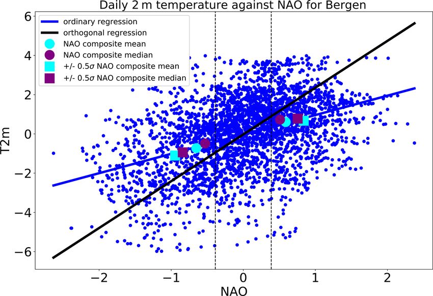
E. Madonna et al.: Reconstructing winter climate using circulation patterns                                                        791

perature reconstruction using regression techniques instead
of composites. Using a simple ordinary linear regression on
daily NAO and temperature values, we find relationships (◦ C
per unit anomalous NAO index) very similar to those found
by the composite method shown in Fig. 4. A reconstruction is
then made by multiplying the regression pattern by the mean
NAO value for each season. In this regression approach, all
days are used in the reconstruction (compared to about half
the days in the composite approach). However, the correla-
tion and CE values of the two reconstructions are very sim-
ilar, and both require a scaling factor to maximize the skill.
This suggests that the need for a scaling factor is not linked
to the omission of information (i.e. the neutral NAO or unde-
fined days).
   If, instead, the regression between daily temperature
                                                                   Figure 11. Illustration of the different regression slopes from ordi-
anomalies and daily NAO values is calculated using a               nary (blue) and weighted orthogonal (black) regression on daily val-
weighted orthogonal distance regression (using the Python          ues of temperature (T2m) the grid box closest to Bergen, Norway,
package scipy.odr), the regression relationship changes – the      plotted against NAO. The cyan (purple) circles and squares show
slope of the linear fit generally increases. An example is         composite mean (median) values for all positive/negative NAO days
shown in Fig. 11 for Bergen (cf. blue regression line for or-      and all positive/negative NAO days with |NAO| > 0.5σ .
dinary least squares, black regression line for orthogonal dis-
tance). This increase in regression slope means that the re-
construction amplitudes increase, and there is less need for a
scaling factor. The weighted orthogonal distance regression        5   Concluding remarks
takes into account “noise” in both the temperature and the
NAO values, while ordinary least squares considers the val-        In this study, we investigate how well seasonal anomalies in
ues of the independent variable (in this case the NAO) to be       European precipitation and temperature can be reconstructed
exact (e.g. Wu and Yu, 2018). This noise may be related to         based on the frequency of circulation patterns defined using
a lag–lead relationship between circulation patterns and sur-      three different classifications: the NAO index, blocking, and
face weather anomalies and/or uncertainty in the connections       the configuration of the North Atlantic jet stream.
between the NAO circulation anomalies and surface temper-             The skill of the various classifications in reconstructing
ature. In Fig. 11 the mean composite values for this grid box      seasonal anomalies depends on the variable and region of
are shown by the cyan markers, and they fall on the ordinary       interest. For the NAO and jet clusters, the regions of high
least squares regression line. The median composite values         skill for precipitation are rather different than for temperature
are also shown in purple, demonstrating that using the com-        (see Fig. 9). Precipitation in western Europe is particularly
posite median would not remove the need for the scaling fac-       well reconstructed, with many coastal and mountainous areas
tor. This suggests that the need for the scaling factor in the     showing coefficient of efficiency values for scaled precipita-
composite and ordinary least squares regression reflects the       tion greater than 0.5 (Fig. 9). For these areas, precipitation
large variability in temperature and precipitation within each     in winter is directly linked to the propagation of storms trav-
classification pattern (cf. Figs. S7 and S8).                      elling from the Atlantic (Hawcroft et al., 2012; Pfahl et al.,
   Finally, the ability to reconstruct precipitation and temper-   2014), which is to first order set by large-scale circulation
ature might be affected by extreme events. For example, if         variability. Still, the relationship between circulation and pre-
a single extreme precipitation event is responsible for the        cipitation is far from straightforward, seen by the fact that
lion’s share of precipitation in a specific season, we would       in some places precipitation is reconstructed with compara-
not expect a skilful reconstruction of the seasonal anomaly        ble (high) skill by all three methods (e.g. Bergen, Norway),
using the average precipitation signals associated with each       while in other places one method performs worse than oth-
basis function. The effect of extreme events varies region-        ers (e.g. NAO in Galicia). For temperature, circulation influ-
ally, as shown for summer temperatures by Röthlisberger            ences the horizontal and vertical advection of air, allowing
et al. (2020). It would therefore be interesting to investigate    a simple index like the NAO to provide skilful reconstruc-
to what extent extreme events influence the seasonal precipi-      tions across much of northern Europe. However, over France
tation and temperature anomalies over Europe and how these         temperatures are better captured by the blocking reconstruc-
events are related to circulation anomalies.                       tion. In southern and inland regions (e.g. Berlin, Germany),
                                                                   none of the methods provides skilful reconstructions of tem-
                                                                   perature or precipitation, suggesting that factors unrelated to
                                                                   circulation are important, for example radiative forcing (e.g.

https://doi.org/10.5194/wcd-2-777-2021                                                Weather Clim. Dynam., 2, 777–794, 2021
792 E. Madonna et al.: Reconstructing winter climate using circulation patterns
clear vs. cloudy, Trigo et al., 2004), soil moisture coupling spectively. We thank two anonymous reviewers for their construc-
(Fischer et al., 2007), or snow–albedo feedback. tive comments that improved the quality of this article.
In the end, no single classification metric emerges as pro-
viding “the best” reconstruction of both precipitation and
temperature across all regions. The three circulation metrics Financial support. This research has been supported by the Re-
– jet clusters, blocking, and NAO – are clearly connected but search Council of Norway (grant no. 276730) and H2020 Marie
emphasize different aspects of the large-scale flow with dif- Skłodowska-Curie Actions (grant no. 797961).
ferent implications for surface climate. The results presented
here can provide guidance on which classification method is
Review statement. This paper was edited by Paulo Ceppi and re-
most suitable for linking regional climate to circulation vari-
viewed by two anonymous referees.
ability. Through this approach, one may gain insight into the
surface impacts of weather events over a range of timescales.
Regime-based reconstruction may prove useful in extended
range predictability (Kim et al., 2016; Scaife et al., 2014)
and in assessing changes in the frequency of weather patterns
References
that constitute the changes in the climatology under anthro-
pogenic forcing. Athanasiadis, P. J., Wallace, J. M., and Wettstein, J. J.: Patterns of
wintertime jet stream variability and their relation to the storm
tracks, J. Atmos. Sci., 67, 1361–1381, 2010.
Code and data availability. ERA-Interim data can be down- Battisti, D. S., Vimont, D. J., and Kirtman, B. P.: 100 Years
loaded from the ECMWF page https://apps.ecmwf.int/datasets/ of progress in understanding the dynamics of coupled atmo-
data/interim-full-daily/levtype=sfc/ (last access: 14 May 2020) sphere/ocean variability, Meteor. Mon., 59, 8.1–8.57, 2019.
(ECMWF, 2020; Dee et al., 2011). The NAO index was down- Briffa, K. R., Jones, P. D., and Schweingruber, F. H.: Tree-Ring
loaded from NOAA ftp://ftp.cpc.ncep.noaa.gov/cwlinks/norm. Density Reconstructions of Summer Temperature Patterns across
daily.nao.index.b500101.current.ascii (last access: 14 May 2020) Western North America since 1600, J. Climate, 5, 735–754,
(NOAA, 2020). The method to identify blocking is described 1992.
in Scherrer et al. (2006) and for jet clusters in Madonna et al. Bürger, G.: On the verification of climate reconstructions, Clim.
(2017). The winter time series used in this study are available at Past, 3, 397–409, https://doi.org/10.5194/cp-3-397-2007, 2007.
https://doi.org/10.5281/zenodo.4011886 (Madonna, 2021). Cassou, C.: Intraseasonal interaction between the Madden–Julian
oscillation and the North Atlantic Oscillation, Nature, 455, 523–
527, 2008.
Supplement. The supplement related to this article is available on- Cattiaux, J., Douville, H., and Peings, Y.: European temperatures
line at: https://doi.org/10.5194/wcd-2-777-2021-supplement. in CMIP5: origins of present-day biases and future uncertainties,
Clim. Dynam., 41, 2889–2907, 2013.
Christiansen, B.: Atmospheric circulation regimes: Can cluster
Author contributions. DSB and EM designed the study. EM per- analysis provide the number?, J. Climate, 20, 2229–2250, 2007.
formed most of the analysis, with RHW contributing the NAO re- Corte-Real, J., Zhang, X., and Wang, X.: Large-scale circulation
gression analysis. All authors contributed to the interpretation and regimes and surface climatic anomalies over the Mediterranean,
discussion of the results and the writing of the paper. Int. J. Climatol., 15, 1135–1150, 1995.
Cortesi, N., Torralba, V., González-Reviriego, N., Soret, A., and
Doblas-Reyes, F. J.: Characterization of European wind speed
Competing interests. Camille Li and David S. Battisti are members variability using weather regimes, Clim. Dynam., 53, 4961–
of the editorial board of the journal. 4976, 2019.
Davini, P., Cagnazzo, C., Fogli, P. G., Manzini, E., Gualdi, S., and
Navarra, A.: European blocking and Atlantic jet stream variabil-
ity in the NCEP/NCAR reanalysis and the CMCC-CMS climate
Disclaimer. Publisher’s note: Copernicus Publications remains
model, Clim. Dynam., 43, 71–85, 2014.
neutral with regard to jurisdictional claims in published maps and
Dee, D. P., Uppala, S. M., Simmons, A. J., Berrisford, P., Poli, P.,
institutional affiliations.
Kobayashi, S., Andrae, U., Balmaseda, M. A., Balsamo, G.,
Bauer, P., Bechtold, P., Beljaars, A. C. M., van de Berg, L.,
Bidlot, J., Bormann, N., Delsol, C., Dragani, R., Fuentes, M.,
Acknowledgements. Erica Madonna and Camille Li acknowledge Geer, A. J., Haimberger, L., Healy, S. B., Hersbach, H.,
funding from the Research Council of Norway (Nansen Legacy Hólm, E. V., Isaksen, L., Kållberg, P., Köhler, M., Matricardi, M.,
grant no. 276730). Rachel H. White received funding from the Eu- McNally, A. P., Monge-Sanz, B. M., Morcrette, J.-J., Park, B.-
ropean Union’s Horizon 2020 research and innovation programme K., Peubey, C., de Rosnay, P., Tavolato, C., Thépaut, J.-N., and
under the Marie Skłodowska-Curie grant agreement no. 797961 and Vitart, F.: The ERA-Interim reanalysis: configuration and perfor-
from the Tamaki Foundation. ECMWF and NOAA are acknowl- mance of the data assimilation system, Q. J. Roy. Meteor. Soc.,
edged for providing the ERA-Interim reanalyses and NAO data, re- 137, 553–597, 2011.
Weather Clim. Dynam., 2, 777–794, 2021 https://doi.org/10.5194/wcd-2-777-2021You can also read