The spatial extent of hydrological and landscape changes across the mountains and prairies of Canada in the Mackenzie and Nelson River basins ...
←
→
Page content transcription
If your browser does not render page correctly, please read the page content below
Hydrol. Earth Syst. Sci., 25, 2513–2541, 2021
https://doi.org/10.5194/hess-25-2513-2021
© Author(s) 2021. This work is distributed under
the Creative Commons Attribution 4.0 License.

The spatial extent of hydrological and landscape changes across the
mountains and prairies of Canada in the Mackenzie and Nelson
River basins based on data from a warm-season time window
Paul H. Whitfield1,2,3 , Philip D. A. Kraaijenbrink4 , Kevin R. Shook1 , and John W. Pomeroy1
1 Centrefor Hydrology, University of Saskatchewan, Saskatoon, SK, S7N 1K2, Canada
2 Department of Earth Sciences, Simon Fraser University, Burnaby, BC, Canada
3 Environment and Climate Change Canada, Vancouver, BC, Canada
4 Geosciences, Utrecht University, Utrecht, the Netherlands

Correspondence: Paul H. Whitfield (paul.h.whitfield@gmail.com)

Received: 24 November 2020 – Discussion started: 4 January 2021
Revised: 30 March 2021 – Accepted: 8 April 2021 – Published: 18 May 2021

Abstract. East of the Continental Divide in the cold inte-       separating the Canadian Rockies and other mountain ranges
rior of Western Canada, the Mackenzie and Nelson River           in the west from the poorly defined drainage basins in the
basins have some of the world’s most extreme and variable        east and north. Three specific areas of change were iden-
climates, and the warming climate is changing the landscape,     tified: (i) in the mountains and cold taiga-covered subarc-
vegetation, cryosphere, and hydrology. Available data consist    tic, streamflow and greenness were increasing while wetness
of streamflow records from a large number (395) of natu-         and snowcover were decreasing, (ii) in the forested Boreal
ral (unmanaged) gauged basins, where flow may be peren-          Plains, particularly in the mountainous west, streamflows
nial or temporary, collected either year-round or during only    and greenness were decreasing but wetness and snowcover
the warm season, for a different series of years between         were not changing, and (iii) in the semi-arid to sub-humid
1910 and 2012. An annual warm-season time window where           agricultural Prairies, three patterns of increasing streamflow
observations were available across all stations was used to      and an increase in the wetness index were observed. The
classify (1) streamflow regime and (2) seasonal trend pat-       largest changes in streamflow occurred in the eastern Cana-
terns. Streamflow trends were compared to changes in satel-      dian Prairies.
lite Normalized Difference Indices.
   Clustering using dynamic time warping, which overcomes
differences in streamflow timing due to latitude or elevation,   1   Introduction
identified 12 regime types. Streamflow regime types exhibit
a strong connection to location; there is a strong distinction   Western Canada, east of the Continental Divide, has extreme
between mountains and plains and associated with ecozones.       and variable climates and is experiencing rapid environmen-
Clustering of seasonal trends resulted in six trend patterns     tal change (DeBeer et al., 2016) where a changing climate
that also follow a distinct spatial organization. The trend      is affecting the landscape, the vegetation, and the water. The
patterns include one with decreasing streamflow, four with       southern part of this region sustains 80 % of Canada’s agri-
different patterns of increasing streamflow, and one with-       cultural production, a large portion of its forest wood, and
out structure. The spatial patterns of trends in mean, min-      pulp and paper production and also includes several glob-
imum, and maximum of Normalized Difference Indices of            ally important natural resources (e.g. uranium, potash, coal,
water and snow (NDWI and NDSI) were similar to each other        petroleum). Understanding both observed changes and possi-
but different from Normalized Difference Index of vegeta-        ble future changes is clearly in the national interest. Climate
tion (NDVI) trends. Regime types, trend patterns, and satel-     variation and change have been demonstrated to have impor-
lite indices trends each showed spatially coherent patterns      tant effects on the rivers of Canada (Whitfield and Cannon,

Published by Copernicus Publications on behalf of the European Geosciences Union.

2514                                         P. H. Whitfield et al.: The spatial extent of hydrological and landscape changes

2000; Zhang et al., 2001; Whitfield et al., 2002; Janowicz,            Streamflow data in this domain are taken from stations
2008; Déry et al., 2009a, b; Tan and Gan, 2015), includ-            that were operated either year-round or seasonally (MacCul-
ing Western Canada’s cold interior (Luckman, 1990; Burn,            loch and Whitfield, 2012); seasonal stations generally pro-
1994; Luckman and Kavanaugh, 2000; Ireson et al., 2015;             vide records from April through the end of October, be-
Dumanski et al., 2015; Ehsanzadeh et al., 2016). The sensi-         cause there is either no streamflow in the winter or because
tivity of streamflow to changes in temperature and precip-          the channels become completely frozen. This approach con-
itation may differ by period of the year (Leith and Whit-           trasts with many studies that use only stations having contin-
field, 1998; Whitfield and Cannon, 2000; Botter et al., 2013).      uous records and a common period of years (e.g. Whitfield
Trends in water storage, based on Gravity Recovery and Cli-         and Cannon, 2000); one novel aspect of this study is that it
mate Experiment (GRACE) satellites, identified precipitation        demonstrates a method which incorporates records from both
increases in northern Canada, a progression from a dry to a         continuous and seasonal stations. Trend assessment is con-
wet period in the eastern Prairies/Great Plains, and an area        ducted on an annual common time window for both continu-
of surface water drying in the eastern boreal forest (Rodell        ous and temporary streams.
et al., 2018). The Mackenzie and Nelson (Saskatchewan                  Landscape changes may cause or result from hydrological
and Assiniboine–Red) River basins were the focus of this            changes. Satellite imagery and derived spectral indices were
study and are where cold-region climatic, hydrological, eco-        used to assess the changes in the landscapes of basins in re-
logical, and cryospheric processes are highly susceptible to        lation to their hydrological response. Normalized Difference
the effects of warming. Both rivers arise in the Canadian           Indices of vegetation, water, and snow (NDVI, NDWI, and
Rockies and receive the vast majority of their runoff from          NDSI) were constructed using optical imagery from the The-
high-elevation headwater basins that are dominated by heavy         matic Mapper (TM) sensor (USGS and NOAA, 1984) on-
snowfall, long-lasting seasonal snowcover, glaciers, and ice-       board the Landsat 5 satellite for individual basins (e.g. Hall
fields. The whole region is subject to strong seasonality, con-     et al., 1995; Su, 2000; Hansen et al., 2013; Pekel et al., 2016).
tinental climate, near absence of winter rainfall, and season-      The temporal coverage of the indices differs from that of the
ally frozen soils. From the mid-boreal forest northwards and        hydrometric data used in this study. Trends in these indices
at high elevations, the surface is an annually thawed active        over many basins from the satellite imagery that is avail-
layer below which materials are permanently frozen (per-            able provides a complementary perspective on hydrological
mafrost). Tens of millions of lakes and wetlands cover the          change over the study domain.
northern and eastern parts of this region, where the Cana-             The objective of this study was to examine the hydrologi-
dian Shield dominates topography and hydrography. Cold              cal structure and changes in seasonal streamflow patterns by
winters and coincidence of the precipitation maximum with           combining data from perennial and temporary streams to di-
the snowmelt period or postmelt period mean that rivers and         agnose hydrological process differences and change across
streams have minimum flows in late winter and maximum               Western Canada’s cold interior. Linking continuous and sea-
flows in late spring. This study provides a statistical assess-     sonal data from a large number of hydrometric stations using
ment of patterns and recent changes in the warm-season hy-          only warm-season data, three important questions were ad-
drological regime and in satellite indices of vegetation, water     dressed in this study domain.
storage, and snow and of the spatial patterns of these changes          1. How are the hydrological types and processes dis-
at gauged basins across this large domain.                                 tributed?
   Hydrological processes differ widely in this domain,
which spans 11 of Canada’s 15 terrestrial ecozones and in-              2. How are climate-related trends distributed?
cludes many small basins where streamflow is only tempo-                3. Are some hydrological types and processes more sus-
rary (Buttle et al., 2012). The hydrographs of all rivers in this          ceptible to change over time?
domain reflect contributions from snowmelt, the magnitudes
of which differ in both space and time. Other flow contribu-           By examining trends in normalized difference indices for
tions, from glaciers and rainfall, all vary spatially across the    basins, this study also addresses whether there are changes
domain, with glacier contributions focussed in high mountain        that may be driving or following the hydrological change be-
headwaters and rainfall contributions increasing at lower ele-      ing observed.
vations and latitudes. Ecozones (Marshall et al., 1999; Eamer
et al., 2014; Ireson et al., 2015) were chosen as an appropri-      2     Methods
ate level for comparisons rather than physical attributes such
as climate, permafrost, or geology, since ecozones represent        2.1    Data
regions where the ecology and physical environment operate
as a system. It is important to note that many rivers in this       The hydrometric (streamflow) stations selected for this study
study originate in one ecozone and cross through other eco-         were all designated as “active” (i.e. were currently moni-
zones whilst maintaining the characteristics of their source.       tored), “natural” (i.e. their flows are not managed), and ei-
                                                                    ther continuous or seasonal and shown as having more than

Hydrol. Earth Syst. Sci., 25, 2513–2541, 2021                                         https://doi.org/10.5194/hess-25-2513-2021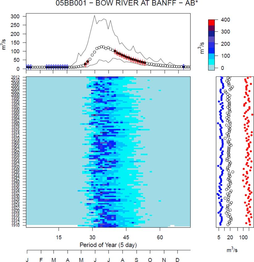
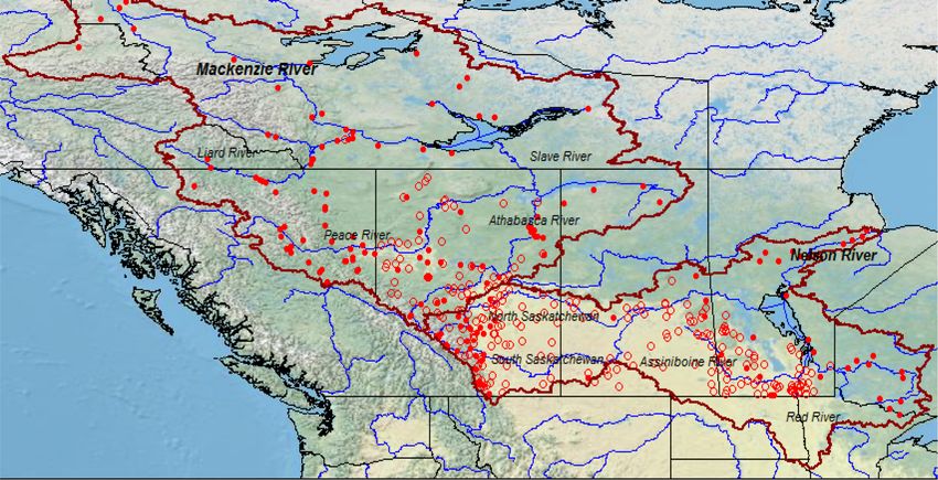
P. H. Whitfield et al.: The spatial extent of hydrological and landscape changes                                             2515

30 years of data in ECDataExplorer (Environment Canada,            the Landsat 5 satellite for each gauged basin. The satellite
2010) at the time the data were downloaded. No attempts            had a 16 d return period between 1985 and 2010 and acquired
were made to use a common window of years – rather all             imagery for any location on the Earth’s surface with a spatial
analyses used the entire period of record for each station.        resolution of 30 m. The sensor was selected for its spectral
In trend studies, time periods are selected that are a trade-      capabilities, which allowed evaluation of surface changes,
off between record length and network density (Hannaford et        and its long operation which best suits the length of the hy-
al., 2013). Many trend studies use a common period of years        drological record in the gauged basins. It was chosen to avoid
with an arbitrary measure of completeness such as 20 years         combining data from different satellites or sensors to main-
of data in a 60-year period (e.g. Vincent et al., 2015) and rely   tain consistency in spectral response over the study period.
on continuous data throughout the year so that measures such       Later satellites use different spectral bands.
as annual mean flow, or specific monthly flows, can be as-
sessed for trend. This generally means that only continuously      2.2   Analysis
observed sites would be included. The alternative approach
used here includes data from a large number of seasonal and        All analyses were performed with R (R Development Core
continuously observed sites, which are compared using only         Team, 2014) using packages kendall (McLeod, 2015),
the data available from April until the end of October.            CSHShydRology (Anderson et al., 2018), and dtwclust
   The locations of the hydrometric stations, the main river       (Sarda-Espinosa, 2017, 2018). A threshold of 0.05 was used
basins, and major tributaries are shown in Fig. 1. Given           in tests of significance, and accordingly, 5 % was also used
the northerly (Mackenzie) or easterly direction of river flow      as an indicator that the number of trends exceeds the number
in the region, the hydrometric stations generally sample           expected by chance alone.
basin hydrology that lies to the south or west of the points          As the intention was to include data from as many sta-
shown. The number of continuous and seasonal stations in           tions as possible, the entire period of record from each of
each of the larger river basins is given in Table 1. Three         the 395 gauged basins was used, and only the window where
additional stations were purposely included: these were at         data were available from every station during the year from
Changing Cold Regions Network (CCRN) Water, Ecosys-                21 April to 1 November was analysed. Table 2 provides the
tem, Cryosphere, and Climate (WECC) observatories, Mar-            starting dates of the 5 d period corresponding to each 5 d pe-
mot Creek, Alberta, Smith Creek, Saskatchewan, and Scotty          riod number from April through November. Because the sta-
Creek, Northwest Territories (Table 1), and including these        tion periods of record were used, rather than a common pe-
stations provides a link between the spatial patterns reported     riod of years, it was not appropriate to compare the magni-
in this study and intensive process-based CCRN studies (De-        tudes of trends among the stations. Instead, the analyses were
Beer et al., 2016, 2021). Streamflow data from a total of 395      restricted to determining the existence of significant trends in
stations (gauged basins) were available; 233 (59 %) were op-       individual 5 d periods from 21 April to 1 November (periods
erated on a seasonal basis. Water Survey of Canada station         23 to 61, Table 2).
numbers are here referred to as stationID. Basin areas range          The main panel in Fig. 2 (bottom left) uses colour to
from 9.1 km2 (Marmot Creek) to 270 000 km2 (Liard River at         show the magnitude of the flow for each day of each year
the mouth) and station elevations range from 22 m (Anderson        for the Bow River at Banff, AB (stationID = 05BB001),
River below Carnwath River) to 2095 m (Mistaya River near          an example of a long and complete continuous streamflow
Saskatchewan Crossing). The data set contains values from          record from a national park in the Canadian Rockies. This
nested basins which may cause some correlations; the anal-         streamflow record was described in detail in Whitfield and
yses performed do not require sites to be statistically inde-      Pomeroy (2016, 2017). The upper panel of Fig. 2 shows the
pendent. Individual stations were analysed for all periods for     minimum, median, and maximum values for each 5 d period
which data were available, but clustering and statistical anal-    and blue (red) arrows indicate periods where there are sig-
ysis involving multiple stations were restricted to the data in    nificant increasing (decreasing) trends in streamflow over the
the annual common time window of the year from 21 April            period of record using Mann–Kendall tests. The directions of
to 1 November when both seasonal and continuous data sets          significant trends (i.e. positive or negative) were determined
were available. Plots of missingness and annual station den-       and were used subsequently for clustering of change types.
sities of the data set are provided in Fig. S1.                    The panel on the right shows the time series of annual mini-
   Satellite imagery and derived spectral indices are valuable     mum, median, and maximum discharges. If there was a sig-
for assessing effects of environmental changes and the hy-         nificant trend (Mann–Kendall τ , p ≤ 0.05), the series was
drological responses of the gauged basins; these methods al-       coloured (red for decreasing, blue for increasing); black for
low determination of changes in vegetation, water bodies and       no trend. The function for generating these plots was from
snowcover for large areas (e.g. Hall et al., 1995; Hansen et       CSHShydRology.
al., 2013; Pekel et al., 2016; Su, 2000). Time series of spec-        The stations in this study were operated for differing peri-
tral remote sensing indices were constructed using optical         ods of time and with differing operating schedules. Figure 3
imagery from the TM sensor (USGS and NOAA, 1984) on                provides an example for the Bow River at Lake Louise, AB

https://doi.org/10.5194/hess-25-2513-2021                                       Hydrol. Earth Syst. Sci., 25, 2513–2541, 2021

2516                                          P. H. Whitfield et al.: The spatial extent of hydrological and landscape changes

Figure 1. Study area showing the Mackenzie and Nelson River basins (dark-red outline) and the location of continuous stations (red dots)
and seasonal stations (red circles). Basemap © OpenStreetMap contributors 2021. Distributed under a Creative Commons BY-SA License.

Table 1. Hydrometric stations included in the analysis. Only stations that are in these three basins were considered; to be included, they
needed to be designated as having natural streamflow, being active, and having more than 30 years of record. The three other hydrometric
stations were associated with a Changing Cold Regions Network Water, Ecosystem, Cryosphere, and Climate (WECC) Observatory with the
number of years of record shown in parentheses.

               Drainage basin               Water Survey    Continuous     Seasonal    Other continuous    Other seasonal
                                            basin code
               Nelson River basin
               Saskatchewan                 05A-05K                  29          98                        05BF016 (50)
               Assiniboine, Red, Nelson     05L-05U                  30          77                        05ME007 (37)
               Mackenzie River basin
               Athabasca                    07A-07D                  22          30
               Peace                        07E-07K                  30          22
               Slave                        07L-07W                  13           4
               Liard                        10A-10E                  22           1    10ED009 (17)
               Mackenzie                    10f-10N                  16           0
                                                                    161         231    1                   2

(05BA001), a station upstream of the Bow River at Banff,               ther since a large proportion of the stations have seasonal op-
showing that this station had continuous operation between             eration. Figures S2–S13 show up to four example hydromet-
1910 and 1920, was discontinued from 1921 until 1963, oper-            ric stations for each streamflow regime cluster, as described
ated continuously between 1964 and 1986, and then had sea-             below. Many of these plots show stations where the operation
sonal operation between 1987 and 2013, hence records only              has alternated between being seasonal and continuous, simi-
exist during the warm season (Fig. 3). The seasonal trends             lar to Fig. 3. Figures S2–S13 also demonstrate the variation
shown in the upper panel are based on all years in which data          in the years of record between stations. The complexity of the
were present in the 5 d periods. In the right-hand panel, trends       data set results from historical budgetary and management
over time in annual minima, medians, and maxima are based              decisions in the Canadian hydrometric program. Assessing
only upon the years with complete data, and this shows gaps            hydrological regimes and trends in this data set requires ap-
in the time series. Trends of these types should be based only         proaches that are different from “standard” methods.
using years with complete records and are not addressed fur-

Hydrol. Earth Syst. Sci., 25, 2513–2541, 2021                                              https://doi.org/10.5194/hess-25-2513-2021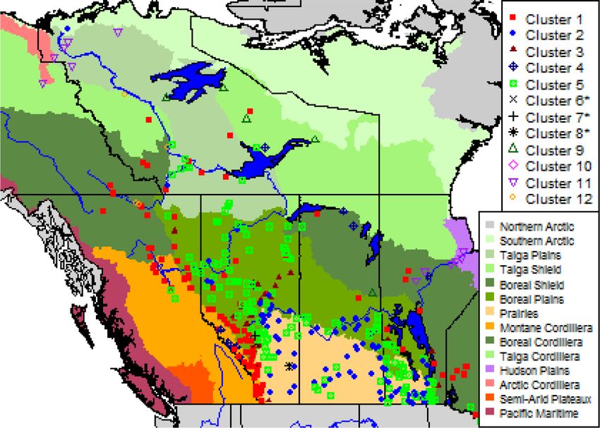
P. H. Whitfield et al.: The spatial extent of hydrological and landscape changes                                                2517

Table 2. Look-up table of 5 d periods during the annual common
time window.

                 5 d period no.   Starting date
                 22               16 Apr
                 23               21 Apr
                 24               26 Apr
                 25               1 May
                 26               6 May
                 27               11 May
                 28               16 May
                 29               21 May
                 30               26 May
                 31               31 May
                 32               5 Jun
                 33               10-Jun
                 34               15 Jun
                 35               20 Jun
                 36               25 Jun
                 37               30 Jun
                 38               5 Jul
                 39               10 Jul
                 40               15 Jul
                 41               20 Jul                          Figure 2. Plot of observed flows in the Reference Hydrologic Basin
                 42               25 Jul                          station 05BB001 Bow River at Banff, Alberta. The main panel
                 43               30 Jul                          shows the 5 d periods of the year against the years of record. White
                 44               4 Aug                           space indicates missing observations and the colours represent flow
                 45               9 Aug                           magnitudes scaled according to the bar in the upper right corner.
                 46               14 Aug                          The upper panel shows the maximum, median and minimum flow
                 47               19 Aug                          for each of the 5 d periods and red (blue) arrows indicate statis-
                 48               24 Aug                          tically significant decreases (increases) using Mann–Kendall τ at
                 49               29 Aug                          p ≤ 0.05. The panel on the right-hand side shows the annual min-
                 50               3 Sep                           ima, median (open circle), and maxima; statistically significant de-
                 51               8 Sep                           creasing (increasing) trends (Mann–Kendall τ at p ≤ 0.05) are in-
                 52               13 Sep                          dicated by red (blue). Whenever the station is a member of the ref-
                 53               18 Sep                          erence hydrologic basin network (RHBN), an ∗ appears at the end
                 54               23 Sep                          of the station name.
                 55               28 Sep
                 56               3 Oct
                 57               8 Oct                           lines in Fig. 4 (5 d periods 23 to 61) were used in the clus-
                 58               13 Oct                          tering (and subsequent trend analysis) reported here. The use
                 59               18 Oct                          of 5 d means is based on previous work (Leith and Whitfield,
                 60               23 Oct                          1998, Déry et al., 2009b) to place the analysis at a common
                 61               28 Oct
                                                                  time step across all sites and to balance the variation in hy-
                 62               2 Nov
                                                                  drologic signatures of basins of different sizes while avoiding
                                                                  information loss that occurs with smoothing at seasonal and
                                                                  monthly time steps (Whitfield, 1998).
2.2.1   Streamflow Regime Types                                      Statistical methods, such as k-means (Likas et al.,
                                                                  2003; Steinley, 2006) or self-organized maps (Kohonen and
To avoid the effects of the areas of the gauged basins, the 5 d   Somervuo, 1998; Hewitson and Crane, 2002; Kalteh et al.,
streamflow records were converted to z-scores by subtracting      2008; Céréghino and Park, 2009; van Hulle, 2012), are un-
the mean value and dividing by the standard deviation of the      able to group hydrographs when they are not aligned in time
series 5 d medians. The resulting series have means of zero       (Halverson and Fleming, 2015). Across the study domain this
and unit variance; plots of these were scaled in magnitude by     is a difficulty, as the timing of snow accumulation and melt
the standard deviations (e.g. Fig. 4). Early snowmelt at low      are strongly affected by both latitude (48 to 69◦ N) and el-
latitudes and elevations resulted in some stations having flow    evation (near sea level to > 2100 m), reflecting the seasonal
events prior to the annual common time window (Fig. 4).           variation in the 0◦ isotherm (Mekis et al., 2020).
Only the data in the periods between the two vertical dashed

https://doi.org/10.5194/hess-25-2513-2021                                       Hydrol. Earth Syst. Sci., 25, 2513–2541, 2021
2518                                             P. H. Whitfield et al.: The spatial extent of hydrological and landscape changes

                                                                         Figure 5. Example of alignment of two time series using dynamic
                                                                         time warping (DTW) from stations 05AC030 Snake Creek near Vul-
                                                                         can, AB, and 10NC001 Anderson River below Carnwath River, NT.

Figure 3. Plot of observed flows in the 05BA001 Bow River at Lake           The clustering of annual median streamflow time se-
Louise, Alberta, a natural flow station. The main panel shows the 5 d    ries was done using dynamic time warping, DTW (Berndt
periods of the year against the years of record. White space indicates   and Clifford, 1994; Wang and Gasser, 1997; Keogh and
missing observations and the colours are scaled according to the bar     Ratanamahatana, 2005), which measures similarity between
in the upper right corner. The upper panel shows the maximum, me-
                                                                         time series that may vary in magnitude and timing by align-
dian and minimum flow for each of the 5 d periods and red (blue)
                                                                         ing the two standardized (zero mean, unit variance) curves in
arrows indicate statistically significant decreases (increases) using
Mann–Kendall τ at p ≤ 0.05. The panel on the right shows the an-         time, essentially matching the shape of inflections to create
nual minima, median (open circle), and maxima; statistically signif-     clusters (Sarda-Espinosa, 2017; Whitfield et al., 2020).
icant decreasing (increasing) trends (Mann–Kendall τ a p ≤ 0.05)            As an example of the DTW alignment, the z-scores of
are indicated by red (blue).                                             the median streamflows from two stations, the semi-arid
                                                                         foothills and grassland-sourced Snake Creek near Vulcan,
                                                                         AB (05AC030), and Arctic tundra-sourced Anderson River
                                                                         below Carnath River, NT (10NC001), are aligned in Fig. 5.
                                                                         The two curves differ in the timing and magnitude of their
                                                                         peaks (Fig. 5a); the DTW distance calculated is a dissimi-
                                                                         larity measure constructed from a warping path based upon
                                                                         the matching of inflections between the two curves (Fig. 5b)
                                                                         essentially matching the shape of inflections and shifting
                                                                         the curves to a common time frame (Fig. 5c). R package
                                                                         dtwclust (Sarda-Espinosa, 2017) implements dynamic
                                                                         time warping to cluster multiple curves based upon their hav-
                                                                         ing similar shapes and inflections and was used for cluster-
                                                                         ing the 395 cases in this study. The timing of inflections does
                                                                         not affect the clustering, so the effects of latitude and ele-
                                                                         vation that often result in misclassification of hydrographs
Figure 4. Standardized median streamflow for 5 d periods from the
                                                                         because of timing differences are avoided. This is important
395 hydrometric stations. The flow from each station was standard-
ized by removing the mean and dividing by the standard deviation.        given the size of the spatial domain considered here. A 12-
Only the period between 21 April and 1 November (indicated by the        cluster solution was chosen; this number of clusters balances
region between the blue dashed lines) is considered, as seasonally       regional separation of similar hydrograph types while avoid-
operated stations have no observations during winter months.             ing producing many types with single stations which rep-
                                                                         resent unique hydrological situations. “Streamflow Regime
                                                                         Type” in the text which follows refers to these 12 clusters.

Hydrol. Earth Syst. Sci., 25, 2513–2541, 2021                                             https://doi.org/10.5194/hess-25-2513-2021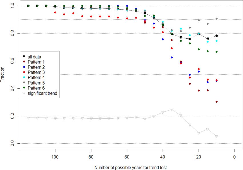
P. H. Whitfield et al.: The spatial extent of hydrological and landscape changes                                            2519

   The centroids of each regime type provide insight into dif-    2.4   Trends in vegetation, water, and snow satellite
ferences in regional hydrology. The shape of the centroid and           indices
the recession slope(s) of the curves provide information that
can be used to further compare differences between clusters.      Given the large study region and the long study period, anal-
                                                                  yses of time series of Landsat 5 TM data are very resource
2.3   Trend Patterns                                              intensive, both in terms of storage and computational power,
                                                                  and are beyond the scope of desktop computing. Google
Trends in each of the 5 d periods for the annual common time      Earth Engine (GEE) allows for cloud-based planetary-scale
window were determined for the period of record of each           analysis, while it serves as a database for petabytes of open-
time series, using Mann–Kendall tests as described above,         access satellite imagery such as the Landsat archive (Gore-
following the approach of Déry et al. (2009b) for examining       lick et al., 2017) and is particularly capable for this study.
trend magnitude for a fixed endpoint in time. Interpreting the       Using GEE, Landsat 5 TM image composites (n = 579)
results for any fixed time period may not be representative       were produced to cover the spatial extent of all the gauged
of a longer timescale (Hannaford et al., 2013). As these were     basins for the period between 1985 and 2010 by mosaicking
comparing periods separated by 360 d, i.e. a resampled time       the available image scenes for each consecutive 16 d period.
series, autocorrelation was not expected, and therefore pre-      Theoretically this would allow for spatially complete mo-
whitening was not applied. Tests with 100+ years of record        saics given the 16 d revisit time of the satellite. To determine
show that nearly 90 % of cases did not show autocorrela-          accurate spectral indices at the basin scale, pixels containing
tion, and the balance was close to the level of significance      clouds or cloud shadows in each image scene were masked
(0.19). The individual station trend test results are indicated   prior to mosaicking using the GEE-integrated Fmask algo-
in the upper panels of Figs. 2, 3, and S2–S13, where sig-         rithm (Zhu et al., 2015), which introduced intermittent data
nificant increases and decreases are indicated by blue and        gaps to the set of mosaics. Additional data gaps were caused
red arrows respectively. The significant increasing, no trend,    by occasional unavailability of satellite image scenes in the
and decreasing trends were assigned scores of 1, 0, and −1        Landsat 5 TM catalogue, typically due to image quality or
respectively. The individual annual trend scores for the an-      georeferencing issues (USGS and NOAA, 1984). To reduce
nual common time window for the 395 stations were clus-           the computation cost and data volume, the final mosaics were
tered using the method of k-means, which partitions obser-        generated at an aggregated spatial resolution of 300 m. The
vations into clusters having similar means and which is well      total number of satellite image scenes used was 83 381.
suited to clustering of features such as patterns of signifi-        For each basin, three time series of spectral index averages
cant differences (Likas et al., 2003; Steinley, 2006; Agarwal     were derived from the 16 d mosaics of Landsat 5 TM data.
et al., 2016). The number of clusters chosen (six) was based      Each normalized difference index (I ) compares two wave-
upon the elbow method (Ketchen and Shook, 1996; Kodi-             length ranges (W 1 and W 2) observed by the satellite detec-
nariya and Makwana, 2013); using more than six clusters did       tors, using the form I = (W 1 − W2)/(W 1 + W 2), each index
not improve the modelling (not shown). These six clusters         ranging between −1 and 1. The three common indices used
are hence referred to as “Trend Patterns”.                        were the Normalized Difference Vegetation Index (NDVI),
   As the method used here is unconventional, we assessed         Normalized Difference Water Index (NDWI), and Normal-
how the patterns of trends would differ when using varying        ized Difference Snow Index (NDSI) (Lillesand et al., 2014)
periods of record. Trends in each of 39 5 d periods were first    and were calculated by
determined for the entire period of record and were then com-
pared to those of 21 periods, with lengths decreasing by 5        NDVI = (RNIR − RRed ) / (RNIR + RRed ) ,                    (1)
years between 1905 and 2005 (e.g. 1905–2015, 1910–2015,           NDWI = (RNIR − RSWIR ) / (RNIR + RSWIR ) , and              (2)
1913–2015). Eleven stations with more than 3 years of data
                                                                  NDSI = (RGreen − RSWIR ) / (RGreen + RSWIR ) ,              (3)
in the final interval (2005–2015) were excluded so that miss-
ing values were not introduced. The ∼ 15 000 comparisons          where R is the dimensionless top-of-atmosphere reflectance,
(384 sites for 39 5 d periods) were used to determine the         Green is TM band 2 (green light 0.52–0.60 µm), Red is TM
number of cases where the trends did not change. These com-       band 3 (red light 0.63–0.69 µm), NIR is TM band 4 (near in-
parisons were also tested using a classification approach and     frared 0.76–0.9 µm), and SWIR is TM band 5 (shortwave in-
the adjusted Rand index (Morey and Agresti, 1985) and pro-        frared 1.55–1.75 µm). Because of the presence of the masked
duced similar results (not provided here).                        cloud pixels and data gaps, the basin means were often only
                                                                  calculated from a fraction of the complete pixel set of the
                                                                  basin; this fraction was determined for every observed time
                                                                  step.
                                                                     For each 16 d period, the mean NDVI, NDWI, NDSI, and
                                                                  fractional coverage were determined for each of 375 gauged
                                                                  basins for which a shapefile of basin boundaries was avail-

https://doi.org/10.5194/hess-25-2513-2021                                      Hydrol. Earth Syst. Sci., 25, 2513–2541, 2021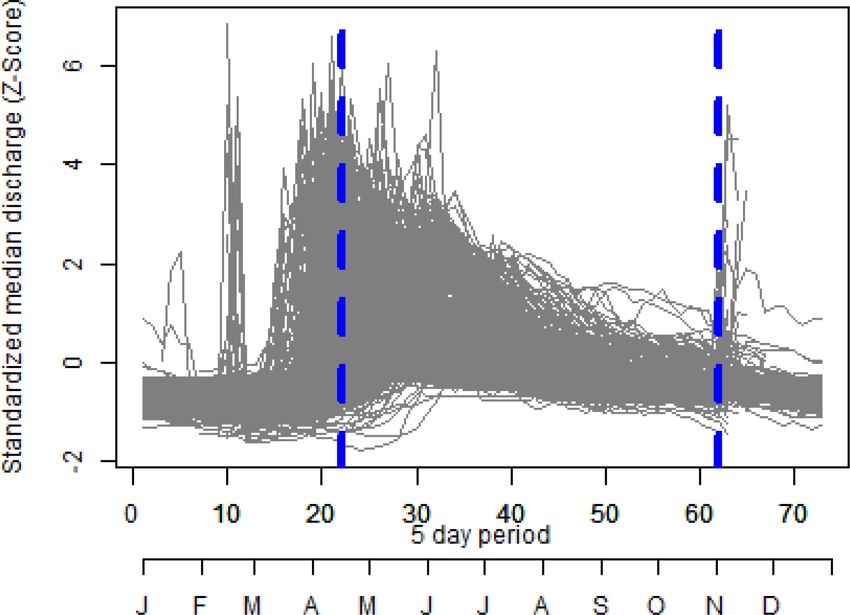
2520                                          P. H. Whitfield et al.: The spatial extent of hydrological and landscape changes

able (20 basin boundaries were not available from Water Sur-         to summer water deficits, variable contributing areas, and
vey of Canada). A sample data set is shown in Fig. S14. Time         frozen conditions in winter (Fig. S3). Streamflow Regime
series of annual maximum, mean, and minimum were deter-              Type 3 basins were in the Athabasca River basin domi-
mined for each of the normalized different indices and their         nated by humid upland boreal forest and lowland muskeg
fractional coverages from these data sets. Since there were          (Fig. S4). Streamflow Regime Type 4 (Fig. S5) has both
only ∼ 22 images (at most) available for each year in each           strong snowmelt and late-summer streamflow. Streamflow
basin, the entire year was used rather than the annual com-          Regime Type 5 basins were predominantly in the sub-humid
mon time window so that the annual minimum, maximum,                 Boreal Plains mixed forest (Fig. S6). Basins of Streamflow
and mean would be comparable across the study domain.                Regime Types 6–8 and 10 were unique (or nearly so) but
   Forkel et al. (2013) demonstrated the annual variability of       were similar to adjacent types (Figs. S7, S8, S9, and S11). An
NDVI time series and the effects of using different analysis         interesting feature of these four types is that peak flows oc-
methodologies. Verbesselt et al. (2010, 2012) and de Jong et         cur at different times in different years. Streamflow Regime
al. (2012) used breaks for additive season and trends (bfast)        Type 9 basins peak later in the summer and were gener-
to detect change, particularly phenological change, in satel-        ally smoother than for other basins (Fig. S10). Streamflow
lite imagery; bfast iteratively estimates the time and number        Regime Type 11 basins have an early snowmelt peak and
of abrupt changes within time series derived from satellite          high flows extending through into the fall (Fig. S12). Stream-
images. While this methodology has considerable appeal and           flow Regime Type 12 basins have an early snowmelt peak
has been used widely and successfully to assess change in            and persistent high flows during summer and extend into the
target areas, it was impractical to apply bfast here as it is dif-   fall (Fig. S13).
ficult to summarize multiple changes in seasonality, trends,            The spatial extents of the 12 Streamflow Regime Types
and breakpoints for three indices across 375 basins. A sim-          were mapped over ecozones in Fig. 7; there is a clear spatial
pler approach, testing for simple trends in the mean, maxi-          organization rather than a random pattern. This association
mum, and minimum indices using Mann–Kendall (McLeod,                 is also evident in Table 3. Two large-scale features are ev-
2015), avoids the rich complexity possible with bfast but            ident: similar types tend to be from the same spatial areas,
still illustrates that NDVI, NDWI, and NDSI changes were             and some similar types follow along major rivers. Stream-
accompanying streamflow regime changes. The minimum                  flow Regime Types 3 and 11 follow along rivers and Types
NDSI values excluded zero values.                                    2 and 5 overlap. Streamflow Regime Types 1 (104 members)
                                                                     and 5 (148) occur in the greatest numbers of ecozones (8 and
                                                                     6 respectively; Table 3).
3     Results                                                           Streamflow Regime Type 1 basins occur in the Cordillera
                                                                     (Montane n = 31 basins, Boreal n = 11, and Taiga n = 1) and
3.1    Streamflow Regime Types                                       also the Boreal Plains (n = 31), Taiga Plains (n = 5), Bo-
                                                                     real Shield (n = 13) and Prairies (n = 11); the Type 1 hy-
The Streamflow Regime Types from the 12-cluster solution             drograph shows a sharp, brief melt period followed by a
are shown in Fig. 6. Each of the 12 plots contains a line for        long, slow recession (Fig. 6). Streamflow Regime Type 5
each gauged basin in that type, and the heavy dashed line,           basins were also common in the Prairie ecozone (n = 49),
where visible, is the centroid of all members; the colour of         in the Boreal Plains (n = 81) as well as along the Macken-
the lines is based upon stationID. The x axis is time, shown         zie River to below Great Slave Lake; the hydrograph for
in increments of 5 d periods; these periods are renumbered           this type shows an earlier and briefer peak than Type 1,
starting with 1 for period 23. The y axis is the z-score (stan-      with a rapid recession (Fig. 6). Streamflow Regime Type
dard deviation units); the series for each site was converted to     4 basins (n = 10) were predominantly found in the Mon-
a z-score subtracting the mean and dividing by the standard          tane Cordillera in the west (n = 5) and in the Boreal Shield
deviation. The differences in the shapes of the hydrographs          and Boreal Plains in the east (n = 2 each); the hydrograph
between regime types are evident and demonstrate how the             shows prolonged high flows during the melt period and a
shapes of the members and locations within a Streamflow              short recession with relatively large flows (Fig. 6). Stream-
Regime Type were similar. The outlying individual cases              flow Regime Type 3 basins (n = 22) appear in the Boreal
(e.g. Streamflow Regime Types 6, 7, and 8) are also evident.         Plains (n = 17), Boreal Shield (n = 2) and Prairies (n = 3)
   Example plots for each of these 12 Streamflow Regime              and demonstrate the persistence of a mountain runoff signal
Types are shown in Figs. S2 to S13 to illustrate the similarity      along the Athabasca River, as this hydrograph contains the
and differences between the hydrographs within the stream-           late-melt signal from glaciers and high-elevation snowpacks
flow regime types. Streamflow Regime Type 1 basins were              (Fig. 6). Streamflow Regime Type 2 basins (n = 85) were as-
generally Rocky Mountain basins that have strong snowmelt            sociated with the Prairie ecozone (n = 57) and Boreal Plains
and spring rainfall maxima signals (Fig. S2). Streamflow             (n = 28), but this pattern also occurs in the Southern Arctic
Regime Type 2 basins were reflective of Prairie streams with         (n = 1) and Taiga Plain (n = 3); this pattern has the earli-
spring snowmelt and long periods with low or zero flow due           est snowmelt and most rapid recession, and the records often

Hydrol. Earth Syst. Sci., 25, 2513–2541, 2021                                        https://doi.org/10.5194/hess-25-2513-2021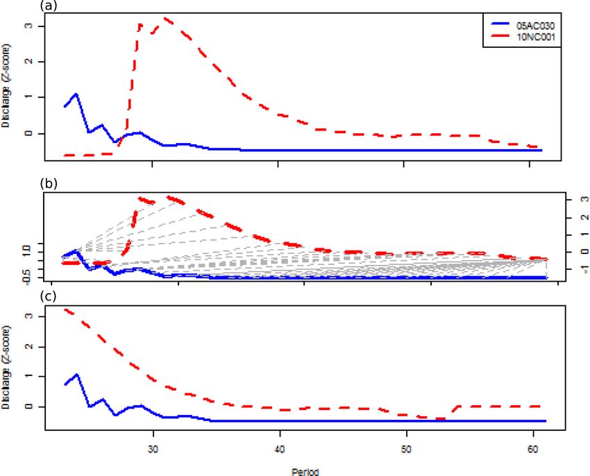
P. H. Whitfield et al.: The spatial extent of hydrological and landscape changes                                                       2521

Figure 6. Streamflow Regime Types produced by clustering of the 395 standardized median 5 d streamflows using dynamic time warping.
The individual lines are coloured based on stationID; the consistency of colour reflects similar spatial locations. The heavy dashed line is
the centroid of the cluster. Note that the number on the x axis is for the aligned series (1–39) as opposed to 23–61. The y-axis value is the
z-score and differs in scale between the panels.

Table 3. Streamflow Regime Type classification in relation to the ecozone in which the station is located.

                                                                 Streamflow Regime Type
                       Ecozone                  1     2     3     4      5    6   7    8    9   10    11     12     n
                       Southern Arctic                1                                                             1
                       Taiga Plains             5     3                  9                  1          5     1     24
                       Taiga Shield             1                 2      1                  3                       7
                       Boreal Shield           13           2     2      6                  1          3           27
                       Boreal Plains           31    28    17     1     81    1   1                               160
                       Prairies                11    53     3           49             1         2                119
                       Montane Cordillera      31                 5      2                                         38
                       Boreal Cordillera       11                                                            2     13
                       Taiga Cordillera         1                                                      1     1      3
                       Hudson Plains                                                                   3            3
                       n                      104    85    22    10    148    1   1    1    5    2    12      4   395

https://doi.org/10.5194/hess-25-2513-2021                                              Hydrol. Earth Syst. Sci., 25, 2513–2541, 2021
2522 P. H. Whitfield et al.: The spatial extent of hydrological and landscape changes
Table 4. Summary of recession slopes amongst the 12 Stream-
flow Regime Types. Units are z-score/length estimated from Fig. 8.
Types with ∗ have only one member and are excluded here. NA
means not available.
Streamflow Recession Recession Recession
regime slope 1 slope 2 slope 3
type
1 −0.22 −0.04 NA
2 Nonlinear
3 −0.22 −0.04
4 −0.16 −0.06
5 −0.22 −0.06 0.00
6∗
7∗
8∗
Figure 7. Locations of the 12 Streamflow Regime Types from the 9 −0.04 NA NA
changing cold-region domain overlain on the ecosystems of West- 10 −0.06 NA NA
ern Canada. Clusters marked with an ∗ have only a single member. 11 −0.22 0.00 −0.04
12 −0.06 NA NA
begin with snowmelt already in progress (Fig. 6). Stream-
flow Regime Type 11 basins (n = 12) were located near the zone was useful, the ecozone is a generalization and does not
mouth of the Mackenzie in the Taiga Plains and in the Hud- always capture hydrological functions in the source areas. In
son Plains along the Nelson River in Manitoba. Streamflow many rivers, the source of runoff lies in the high mountains,
Regime Type 12 basins (n = 4) were in the Boreal Cordillera. and these patterns are transmitted along the downstream river
Streamflow Regime Type 6–8 basins (1 each) and 9 (n = 2) course such as in the Mackenzie, Liard, Athabasca, and Nel-
were located at the edges of ecozones. While these descrip- son rivers. Such stations are not independent. Differences be-
tions are explicit, there was overlapping of types in space tween Streamflow Regime Type 1 and 4 basins likely reflect
(particularly Streamflow Regime Types 2 and 5) and cases low late-summer flows from parts of the Rocky Mountains.
where individual basins of a type occur quite separately from In areas where there was overlap between different Stream-
each other (Types 9 and 12), as is evident in Fig. 7. flow Regime Types, both similarities and differences exist
The standardized streamflows plotted in Fig. 6 make it dif- between the basins.
ficult to compare the Streamflow Regime Types; plotting the
z-score centroids of each (Fig. 8) makes the comparisons 3.2 Trend Patterns
simpler. The non-Prairie Streamflow Regime Types have ap-
proximately linear recessions with two slopes (Types 1, 3, Trend Patterns are based upon the statistical trends in 5 d
4, and 12) or more (Type 11). The slopes of the recessions flows discussed above. Figure 9 illustrates the trend results
are listed in Table 4. Typically, the first recession phase was for one station, 05DA007 Mistaya River near Saskatchewan
steeper than the second phase – where there was one. In Crossing, which drains a heavily glaciated mountain basin
Streamflow Regime Type 11 the third phase was steeper than that is undergoing deglaciation. In the case of Fig. 9 there
the second but not as steep as the first. After a rapid recession, were three periods (39, 40, and 46) in July and August with
Streamflow Regime Type 2 becomes nearly horizontal, prob- significant decreases; the other periods have no trends.
ably due to Prairie streams typically having no base flows due Figure 10 plots all significant trends for the 395 basins,
to lack of groundwater contributions. In Streamflow Regime with significant increases and decreases shown in blue and
Type 5 the recession has two linear phases and also termi- red, no trend in gray, and no available data in white. These
nates in a horizontal section, which was again likely to be data were ordered by the six Trend Patterns determined us-
caused by the absence of base flows in many Prairie basins. ing only the data for the 5 d periods from 23 to 61; Fig. S15
These recessions appear to have only five values, two that shows the data order by stationID. Periods 1–22 and 62–73
were steep (−0.22 and −0.16) and two that were much flat- were not included in the clustering but were plotted as they
ter (−0.06 and −0.04) in addition to the zero slope (no slope) are also of interest.
of Type 5. Trend Patterns in Fig. 10 are presented in the order that
A caution is warranted here. The shapes of hydrographs clusters were formed, showing the distinctly different Trend
are controlled by the climate, hydrological processes and Patterns 1, 2, 3, 4, and 6, while Trend Pattern 5, the largest
landscape predominantly in the area of the basin where most group with more than 250 basins (64 % of the total), does not
of the runoff is generated, and while association with an eco- have a consistent organized change despite there being indi-
Hydrol. Earth Syst. Sci., 25, 2513–2541, 2021 https://doi.org/10.5194/hess-25-2513-2021P. H. Whitfield et al.: The spatial extent of hydrological and landscape changes 2523
Figure 8. Centroids of the 12 Streamflow Regime Type clusters.
vidual periods with increasing or decreasing trends. Trend
Pattern 1 shows positive streamflow trends in most of the
annual common time window, suggesting a general increase
in wetness throughout the spring, summer, and fall. Trend
Pattern 2 has positive trends, suggesting increased wetness
after period 30 in early summer. Trend Pattern 3 has pre-
dominantly significant negative trends, with many more in
periods 40–61 than in periods 23–39, suggesting decreases
in late-summer and fall streamflow. Trend Pattern 4 has sig-
nificant increases centred about period 35, suggesting a shift
increased snowmelt and rainfall-runoff peaks in June. Trend
Pattern 6 shows significant increases in the first periods and
last periods of the window but not during the summer; this
group of stations all have winter data and show increasing
streamflow throughout the late fall, winter, and early spring
Figure 9. Example of the trend portion of the summary hydrograph: periods.
the two dashed lines indicate the start and end of the common win- The trends presented in Fig. 10 are based on 39 5 d pe-
dow from period 23 to period 61. riods using the available data seta with records of at least
30 years. The stability of the trend results with decreasing-
length observation periods is demonstrated in Fig. 11, where
https://doi.org/10.5194/hess-25-2513-2021 Hydrol. Earth Syst. Sci., 25, 2513–2541, 20212524 P. H. Whitfield et al.: The spatial extent of hydrological and landscape changes
Figure 11. The fraction of stations with the same Trend Pattern as
in the original full-length record for period lengths decreasing from
115 to 10 years in 5-year steps. The fraction for all data is plotted as
filled black squares and for each of the six Trend Patterns as filled
circles (colours are as in other figures). The fraction of stations with
a significant trend for each step is plotted as gray triangles. This
analysis was done using 384 sites of the original 395; the 11 sites
omitted had less than 3 years’ worth of observed values in the final
Figure 10. Trend patterns in the 395 stations, significant increases
time period (2005–2015).
(blue) and significant decreases (red), no trend (gray) and missing
(white). The stations are ordered by Trend Pattern (cluster) number
and stationID. Data outside the dashed lines were not used in the Table 5. Trend Patterns for 395 stations against their Streamflow
clustering but are shown where available (periods 1–22 and 62–73). Regime Type classification.
Trend Pattern
the trends are compared for increasingly shorter time periods 1 2 3 4 5 6 n
with the results for the entire period. The fraction of the ap- Streamflow 1 1 2 5 13 75 8 104
proximately 15 000 reduced-period results that are the same Regime 2 9 10 10 16 39 1 85
as the complete-period results is greater than 0.75, even when Type 3 2 2 17 1 22
the record length is reduced to 10 years. The mean fraction 4 1 9 10
of sites showing significant trends detected in each time pe- 5 6 10 13 17 101 1 148
riod is about 0.20 and is at a maximum at 35 years and de- 6 1 1
creases at shorter time intervals (Fig. 11). For a period of 10 7 1 1
years, 5 % of the cases show significant trends, as would be 8 1 1
9 1 1 3 5
expected by chance alone (based on a p value of ≤ 0.05). The
10 2 2
impact of reduced length affects the Trend Patterns differ- 11 8 4 12
ently. Trend Patterns 1 to 3 show greater changes in the frac- 12 1 3 4
tion of significant trends than Trend Patterns 4 to 6 (Fig. 11).
n 19 22 32 50 254 18 395
Associating a Trend Pattern with a Streamflow Regime
Type is complicated as there were different numbers of
basins in the Streamflow Regime Types and Trend Patterns
(Table 5). Trend Pattern 5, which lacks any pattern, was very located at the eastern and western margins of the Prairies
prominent in most of the Streamflow Regime Types having with two north of 60◦ , all showing increasing streamflows
many members. Again, the caution regarding rivers sourced throughout the entire year. Trend Pattern 2 (n = 22, S17)
in the mountains and propagating the upstream signal down- basins, with early summer increases, were located across the
stream in nested basins also applies to their Trend Pattern as Prairies and in the eastern portion of the Boreal Plain. Trend
well. Pattern 3 (n = 32, S18) basins, showing decreased stream-
The six Trend Patterns of the 395 hydrometric stations are flow, were located predominantly in the western portions of
mapped to ecozones in Fig. 12. Supplement Figs. S16–S21 the Boreal Plain and on the eastern edge of the Montane
provide more detail on the individual Trend Patterns and the Cordillera. Trend Pattern 4 (n = 50, S19) basins, with larger
station locations. Trend Pattern 1 (n = 19, S16) basins were early summer peaks, were located across the Prairies largely
Hydrol. Earth Syst. Sci., 25, 2513–2541, 2021 https://doi.org/10.5194/hess-25-2513-2021P. H. Whitfield et al.: The spatial extent of hydrological and landscape changes 2525
Table 6. Trend Patterns in relation to the ecozone in which the sta-
tion is located.
Trend Pattern
Ecozone 1 2 3 4 5 6 n
Southern Arctic 1 1
Taiga Plains 1 2 1 13 7 24
Taiga Shield 1 1 4 1 7
Boreal Shield 1 1 3 21 1 27
Boreal Plains 3 9 21 13 114 160
Prairies 14 10 7 29 58 1 119
Montane Cordillera 2 4 32 38
Boreal Cordillera 9 4 13
Taiga Cordillera 3 3
Hudson Plains 3 3
Figure 12. Trend Patterns (colour) and Streamflow Regime Types n 19 22 32 50 254 18 395
(cluster no. with symbols) of the 395 stations in the study domain.
The ecozone legend is as in Fig. 7.
3.3 Trends in vegetation, water, and snow satellite
indices
along the northern edge adjacent to the Boreal Plains and in
a few northern locations in the Boreal Plain. Trend Pattern 5
The spatial patterns of trends in the mean values of the
(n = 254, S20) does not show an organized change pattern in
three normalized difference indices are presented in Fig. 13.
the annual common time window and was distributed across
The spatial patterns of the trends in the maximum, mean,
all the ecozones. Trend Pattern 6 (n = 18, S21) basins, with
and minimum of NDVI, NDWI, and NDSI are provided in
higher cold and cool season flows, were located entirely in
Figs. S22–S24 and are also summarized in comparison with
northern areas in the Taiga Plains, Taiga Shield, and Taiga
Streamflow Regime Type (Table 7), Trend Pattern (Table 8),
and Boreal Cordillera. Overall, 28 % of the basins show one
and ecozone (Table 9). The tables show the fractions of sta-
of the four increasing Trend Patterns, and 8 % have the single
tions grouped by trends that were significant at p ≤ 0.05. In
decreasing pattern.
the figures significant trends (p ≤ 0.05) are shown as red (de-
At the ecosystem scale, 51 % of basins in the Prairies ex-
creasing) or blue (increasing) triangles, trends whose signif-
hibit a definite Trend Pattern, with 45 % showing one of the
icance was ≤ 0.10 are shown as red or blue dots, and those
increasing patterns (Trend Patterns 1, 2, 4, and 6) and 6 %
with no trend are plotted in black. There was a stronger as-
the decreasing Trend Pattern 3 (Table 6). In the Taiga, in-
sociation of the trends in the three indices with spatial loca-
creasing Trend Patterns predominate, with 46 % of stations in
tion and with ecozones than with Streamflow Regime Type
the Taiga Plains showing increasing patterns and none with
or Trend Pattern. Frequently, the trends in vegetation, water,
the decreasing Trend Pattern, 29 % of the Taiga Shield hav-
and snow satellite indices occur in a spatial domain that fol-
ing an increasing Trend Pattern and 14 % a decreasing Trend
lows the margin between two or more ecozones (Figs. 13 and
Pattern, and all three of the Taiga Cordillera basins having
S22–S24).
increasing Trend Patterns (Table 6). The Boreal Shield and
Plains have increasing Trend Patterns in 16 % of stations and 3.3.1 NDVI
decreasing Trend Patterns in 13 %. The Boreal and Mon-
tane Cordillera have increasing Trend Patterns in 11 % of The fractions of stations having statistically significant trends
basins, and only the Montane Cordillera had the decreasing in NDVI were greater than the 5 % expected by chance alone
Trend Pattern (5 %) (Table 6). Trend Pattern 6 only occurs for most Streamflow Regime Types, as listed in Table 7,
in the northern portion of the study area, which is dominated which shows the combinations of increasing and decreasing
by thawing permafrost. None of the stations on the Hudson trends and each trend separately. For example, the fraction
Plains showed any Trend Pattern. These results indicate that of all significant trends for maximum NDVI exceeds 5 % in
the streamflow regime change has a spatial basis, influenced Streamflow Regime Types 1, 2, 3, 5, 9, and 10. The frac-
by the location and ecozone, rather than by the Streamflow tion of significant decreasing trends for maximum NDVI was
Regime Type. greater than 5 % for Streamflow Regime Types 1, 3, 5, 9,
and 10. The fraction of increasing trends in maximum NDVI
exceeds 5 % in Streamflow Regime Types 1, 2, and 5. All
significant trends in mean NDVI were increasing and occur
in Streamflow Regime Types 1, 9, 11, and 12. Significant
https://doi.org/10.5194/hess-25-2513-2021 Hydrol. Earth Syst. Sci., 25, 2513–2541, 20212526 P. H. Whitfield et al.: The spatial extent of hydrological and landscape changes
Table 7. Trends in satellite indices in relation to Streamflow Regime Type. The numbers are the fraction of stations showing a trend; values
greater than 0.05 are in bold.
All changes Stations NDVI max NDVI mean NDVI min NDWI max NDWI mean NDWI min NDSI max NDSI mean NDSI min
1 99 0.15 0.09 0.10 0.03 0.07 0.15 0.03 0.07 0.16
2 79 0.22 0.03 0.18 0.05 0.14 0.15 0.06 0.04 0.06
3 21 0.14 0.05 0.10 0.05 0.10 0.29 0.05 0.00 0.29
4 10 0.00 0.00 0.30 0.00 0.10 0.40 0.00 0.10 0.20
5 142 0.19 0.04 0.11 0.06 0.10 0.18 0.08 0.03 0.09
6 1 0.00 0.00 0.00 0.00 0.00 0.00 0.00 0.00 0.00
7 1 0.00 0.00 0.00 0.00 0.00 0.00 0.00 0.00 0.00
8 0
9 5 0.20 0.40 0.00 0.20 0.40 0.20 0.20 0.40 0.20
10 2 0.50 0.00 0.00 0.00 0.00 0.00 0.00 0.00 0.50
11 12 0.00 0.42 0.25 0.25 0.42 0.25 0.17 0.42 0.25
12 3 0.00 0.67 0.33 0.33 0.33 0.33 0.33 0.33 0.33
Decreases
1 99 0.05 0.03 0.04 0.02 0.05 0.08 0.02 0.07 0.08
2 79 0.03 0.01 0.18 0.00 0.00 0.00 0.00 0.00 0.01
3 21 0.14 0.00 0.05 0.00 0.05 0.14 0.00 0.00 0.10
4 10 0.00 0.00 0.10 0.00 0.10 0.30 0.00 0.10 0.10
5 142 0.13 0.02 0.09 0.01 0.01 0.09 0.01 0.00 0.05
6 1 0.00 0.00 0.00 0.00 0.00 0.00 0.00 0.00 0.00
7 1 0.00 0.00 0.00 0.00 0.00 0.00 0.00 0.00 0.00
8 0
9 5 0.20 0.00 0.00 0.20 0.40 0.20 0.20 0.40 0.20
10 2 0.50 0.00 0.00 0.00 0.00 0.00 0.00 0.00 0.00
11 12 0.00 0.00 0.00 0.25 0.42 0.08 0.17 0.42 0.08
12 3 0.00 0.00 0.00 0.33 0.33 0.00 0.33 0.33 0.00
Increases
1 99 0.10 0.06 0.06 0.01 0.02 0.07 0.01 0.00 0.08
2 79 0.19 0.01 0.00 0.05 0.14 0.15 0.06 0.04 0.05
3 21 0.00 0.05 0.05 0.05 0.05 0.14 0.05 0.00 0.19
4 10 0.00 0.00 0.20 0.00 0.00 0.10 0.00 0.00 0.10
5 142 0.06 0.01 0.01 0.05 0.08 0.09 0.07 0.03 0.04
6 1 0.00 0.00 0.00 0.00 0.00 0.00 0.00 0.00 0.00
7 1 0.00 0.00 0.00 0.00 0.00 0.00 0.00 0.00 0.00
8 0
9 5 0.00 0.40 0.00 0.00 0.00 0.00 0.00 0.00 0.00
10 2 0.00 0.00 0.00 0.00 0.00 0.00 0.00 0.00 0.50
11 12 0.00 0.42 0.25 0.00 0.00 0.17 0.00 0.00 0.17
12 3 0.00 0.67 0.33 0.00 0.00 0.33 0.00 0.00 0.33
375
trends in minimum NDVI were predominantly decreasing in trends with ecozones than with either Streamflow Regime
Streamflow Regime Types 2 and 5 and increasing in Stream- Types or Trend Patterns. Increasing trends in mean NDVI
flow Regime Types 1, 11, and 12 and both increasing and occur in the Taiga Plains, Taiga Shield, Boreal Shield, Bo-
decreasing trends in Streamflow Regime Type 4. real Cordillera and Taiga Cordillera ecozones; decreasing
There were also more significant trends in NDVI than trends in mean NDVI were found more often than expected
would be expected by chance alone in all Trend Patterns (Ta- by chance alone in the Montane Cordillera (Fig. 13a and Ta-
ble 8). The fraction of basins having significant trends in ble 9). The spatial patterns of trends in mean NDVI were sim-
maximum NDVI exceeds 5 % in all Trend Patterns, except ilar to those of the maximum and minimum NDVI (Fig. S23);
Trend Pattern 3, which had no basins with significant trends. however, there were more basins with significant trends in
All mean NDVI trends were increasing and occur only in maximum and minimum NDVI than for mean NDVI. Basins
Trend Patterns 1, 4, and 6. Minimum NDVI trends were pre- with significant increasing trends in maximum NDVI were
dominantly decreasing in all six patterns and increasing in found in the western portion of the Prairies and in the Boreal
Trend Patterns 4 and 6. Shield (Fig. S22a and Table 9); decreasing trends in maxi-
The associations of trends in mean NDVI between 1985 mum NDVI were found in the southern portion of the Boreal
and 2010 with ecozones are each shown in Figs. 13a and Plains, the eastern Prairies, and the southern Boreal Plains
S22 and Table 9. There was a stronger association of NDVI and Boreal Shield (Fig. S22a). The Taiga Plains has basins
Hydrol. Earth Syst. Sci., 25, 2513–2541, 2021 https://doi.org/10.5194/hess-25-2513-2021P. H. Whitfield et al.: The spatial extent of hydrological and landscape changes 2527
Table 8. Changes in satellite indices by Trend Pattern. The numbers are the fraction of stations showing a trend; values greater than 0.05 are
in bold.
All changes Stations NDVI max NDVI mean NDVI min NDWI max NDWI mean NDWI min NDSI max NDSI mean NDSI min
1 17 0.18 0.12 0.29 0.12 0.18 0.18 0.12 0.06 0.18
2 22 0.36 0.00 0.23 0.05 0.14 0.09 0.14 0.09 0.09
3 30 0.00 0.00 0.07 0.10 0.07 0.03 0.13 0.03 0.03
4 47 0.36 0.09 0.15 0.09 0.15 0.21 0.09 0.06 0.04
5 243 0.14 0.05 0.10 0.05 0.09 0.21 0.04 0.04 0.15
6 16 0.06 0.44 0.25 0.06 0.38 0.06 0.06 0.38 0.25
Decreases
1 17 0.12 0.00 0.29 0.12 0.06 0.00 0.12 0.06 0.00
2 22 0.14 0.00 0.23 0.00 0.00 0.05 0.00 0.05 0.05
3 30 0.00 0.00 0.07 0.00 0.00 0.00 0.00 0.00 0.00
4 47 0.06 0.00 0.09 0.02 0.02 0.02 0.02 0.02 0.04
5 243 0.09 0.03 0.07 0.02 0.04 0.11 0.01 0.03 0.07
6 16 0.00 0.00 0.06 0.06 0.38 0.00 0.06 0.38 0.00
Increases
1 17 0.06 0.12 0.00 0.00 0.12 0.18 0.00 0.00 0.18
2 22 0.23 0.00 0.00 0.05 0.14 0.05 0.14 0.05 0.05
3 30 0.00 0.00 0.00 0.10 0.07 0.03 0.13 0.03 0.03
4 47 0.30 0.09 0.06 0.06 0.13 0.19 0.06 0.04 0.00
5 243 0.05 0.02 0.04 0.02 0.05 0.10 0.03 0.01 0.07
6 16 0.06 0.44 0.19 0.00 0.00 0.06 0.00 0.00 0.25
375
with both significant increasing and decreasing trends in min- creasing trends in mean NDWI in Streamflow Regime Types
imum NDVI, and decreasing trends were found at greater 9, 11, and 12.
than expected by change alone in the Taiga Shield, Boreal There were more significant trends in NDWI than would
Plains, and Prairies (eastern); increasing trends were found be expected by chance alone for all Trend Patterns (Table 8).
in the Boreal Shield, Montane Cordillera, Boreal Cordillera, Significant decreasing trends in maximum NDWI exceed the
and Taiga Cordillera (Fig. S22c). Basins with significant threshold 5 % in Trend Patterns 1 and 6, and increasing trends
trends were not randomly distributed through any ecozone, in Trend Patterns 3 and 4 (Table 8). Decreasing trends in
as spatial clustering was evident in each of the three NDVI mean NDWI exceed 5 % in Trend Patterns 1 and 6, as do
trends in Fig. S22. increasing trends in Trend Patterns 1 to 5. The fraction of
basins with decreasing trends in minimum NDWI exceeded
5 % in Trend Pattern 5 and for increasing trends in Trend Pat-
3.3.2 NDWI terns 1, 4, 5, and 6. Only Trend Pattern 5, i.e. without a Trend
Pattern, was found to have both increasing and decreasing
There were more significant trends in NDWI (i.e. hydrologi- trends in minimum NDWI.
cal storage) than would be expected by chance alone in most The associations of trends in mean NDWI with ecozones
Streamflow Regime Types (Table 7), and they were more are shown in Fig. 13b, and Table 9 (Fig. S23 shows re-
prominent in the mean and minimum NDWI than in maxi- sults for maximum, mean, and minimum NDWI). Similar
mum NDWI. Significant trends in maximum NDWI exceed to NDVI, there was a stronger spatial association of NDWI
5 % in Types 2, 5, 9, 11, and 12 with Streamflow Regime trends with ecozones than with either Streamflow Regime
Types 9, 11, and 12 showing increasing trends much greater Types or Trend Patterns. Decreasing trends in mean NDWI
than the threshold (> 20 %), while Streamflow Regime Types occur in the northern ecozones (Taiga Plains, Taiga Shield,
2, 3, and 5 show decreasing trends in about 5 % of the sta- Boreal Cordillera, and Taiga Cordillera; Figs. 13b and S23b);
tions. Significant trends in mean NDWI include both decreas- increasing trends in mean NDWI occur only in the Prairies
ing trends in Streamflow Regime Types 1, 3, 4, 9, 11, and and Boreal Plains. There were more significant trends in
12 and increasing trends in Streamflow Regime Types 2, 3, mean NDWI than in either maximum or minimum NDWI,
and 5. Significant trends in minimum NDWI were decreas- but the spatial patterns for mean NDWI trends were simi-
ing in Streamflow Regime Types 9 and 11 and increasing in lar to those for maximum and minimum NDWI. Basins with
Streamflow Regime Types 2 and 12, with both increasing and significant increasing trends in maximum NDWI were found
decreasing trends in Streamflow Regime Types 1, 3, 4, and 5. only in the western portion of the Prairies and the Boreal
The largest fraction of significant trends (> 33 %) were de- Shield (Fig. S23a and Table 9); decreasing maximum NDWI
https://doi.org/10.5194/hess-25-2513-2021 Hydrol. Earth Syst. Sci., 25, 2513–2541, 2021You can also read