Crustal structure of the Hatton and the conjugate east Greenland rifted volcanic continental margins, NE Atlantic
←
→
Page content transcription
If your browser does not render page correctly, please read the page content below

JOURNAL OF GEOPHYSICAL RESEARCH, VOL. 114, B02305, doi:10.1029/2008JB005856, 2009
  Click
  Here
    for
 Full
Article

Crustal structure of the Hatton and the conjugate east Greenland
rifted volcanic continental margins, NE Atlantic
Robert S. White1 and Lindsey K. Smith1,2
Received 6 June 2008; revised 28 October 2008; accepted 12 November 2008; published 13 February 2009.

[1] We show new crustal models of the Hatton continental margin in the NE Atlantic
using wide-angle arrivals from 89 four-component ocean bottom seismometers deployed
along a 450 km dip and a 100 km strike profile. We interpret prominent asymmetry
between the Hatton and the conjugate Greenland margins as caused by asymmetry in the
initial continental stretching and thinning, as ubiquitously observed on ‘‘nonvolcanic’’
margins elsewhere. This stretched continental terrain was intruded and flooded by
voluminous igneous activity which accompanied continental breakup. The velocity
structure of the Hatton flank of the rift has a narrow continent-ocean transition (COT)
only 40 km wide, with high velocities (6.9 – 7.3 km/s) in the lower crust intermediate
between those of the continental Hatton Bank on one side and the oldest oceanic crust on
the other. The high velocities are interpreted as due to intrusion of igneous sills which
accompanied the extrusion of flood basalts at the time of continental breakup. The
variation of thickness (h) and P wave velocities (vp) of the igneous section of the COT and
the adjacent oceanic crust are consistent with melt formation from a mantle plume with a
temperature 120–130°C above normal at breakup, followed by a decrease of 70–80°C
over the first 10 Ma of seafloor spreading. The h-vp systematics are consistent with the
dominant control on melt production being elevated mantle temperatures, with no
requirement for either significant active small-scale mantle convection under the rift or of
the presence of significant volumes of volatiles or fertile mantle.
Citation: White, R. S., and L. K. Smith (2009), Crustal structure of the Hatton and the conjugate east Greenland rifted volcanic
continental margins, NE Atlantic, J. Geophys. Res., 114, B02305, doi:10.1029/2008JB005856.

1. Introduction                                                            intruded as igneous rocks into the lower crust on the
                                                                           continent-ocean transition [White et al., 2008].
  [2] The description of some continental margins as ‘‘vol-
                                                                             [3] The northern North Atlantic can be considered as the
canic’’ is intended to convey the fact that continental                    type example of volcanic rifted margins. There have been
breakup was accompanied by the eruption of huge volumes                    extensive studies of the continental margins on both sides of
of basaltic lavas. Such margins stand in distinction to                    the North Atlantic, particularly using seismic methods and
nonvolcanic margins that exhibit only minor, or restricted                 by drilling (DSDP leg 12 [Laughton et al., 1972]; DSDP leg
igneous activity at the time of continental breakup. In one                81 [Roberts et al., 1984]; ODP leg 152 [Saunders et al.,
sense the distinction between volcanic and nonvolcanic                     1998]; ODP leg 163 [Larsen et al., 1999]). This means that
margins is unhelpful because there is some igneous activity                there are now several studies of the continental margins in
on all rifted margins; indeed, by the time that seafloor spread-           approximately conjugate locations on either side of the
ing has started, the crust adjacent to all rifted margins is 100%          ocean basin [e.g., Hopper et al., 2003; Smith et al., 2005;
igneous, as it generates oceanic crust. But the volcanic versus            Voss and Jokat, 2007]. In this paper we report new crustal
nonvolcanic distinction remains useful in places like the                  structure results from a pair of strike and dip profiles with
northern North Atlantic, where continental breakup between                 dense deployments of ocean bottom seismometers (OBS)
Greenland and northwest Europe was accompanied by the                      across the Hatton Bank margin west of Rockall (Figure 1)
production of large volumes of flood basalts which flowed                  that provide control on the structure from wide-angle data
across the continental hinterlands on both sides of the new                with unprecedented density and number of arrivals. The
ocean basin. In the case of the northern North Atlantic, the               Hatton profile is approximately conjugate to the SIGMA-3
volume of the extrusive lavas reached more than 1  106 km3                profile across the Greenland continental margin [Holbrook
[White and McKenzie, 1989; Coffin and Eldholm, 1994;
                                                                           et al., 2001; Korenaga et al., 2002; Hopper et al., 2003].
Eldholm and Grue, 1994], with at least as much again
                                                                           Both the Greenland and Hatton Bank profiles extend more
   1
                                                                           than 150 km across the adjacent oceanic crust, so provide an
       Bullard Laboratories, University of Cambridge, Cambridge, UK.       opportunity to map the structure from the continental block,
   2
       Now at BP, Aberdeen, UK.
                                                                           across the continent-ocean transition (COT) and into oce-
Copyright 2009 by the American Geophysical Union.                          anic crust formed by mature seafloor spreading. Comparison
0148-0227/09/2008JB005856$09.00                                            of the Hatton Bank structure from previous seismic studies

                                                                       B02305                                                    1 of 28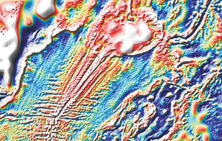
B02305                             WHITE AND SMITH: HATTON CONTINENTAL MARGIN                                            B02305

made in the late 1980s [White et al., 1987; Spence et al., 1989;     [6] The OBS were spaced 4 km apart in the vicinity of
Fowler et al., 1989; Morgan et al., 1989] with the conjugate       the intersection of the main dip and strike lines, with the
Greenland structure show marked asymmetry [Hopper et al.,          spacing increased to 10 km elsewhere (circles, Figure 1).
2003; Smith et al., 2005]. Similar asymmetry has been reported     All the OBS were provided by Geopro, and comprised a
from conjugate margins north of Iceland [Voss and Jokat,           hydrophone with a gimballed type SM-6, 4.5 Hz three-
2007]. In this paper we report recent, detailed studies of the     component geophone. Data were recorded digitally at 4
Hatton margin and then examine the nature of this asymmetry        ms sample rate using a 24-bit analog-digital converter
with the conjugate margin and discuss possible causes for it.      with 120 dB dynamic range. Although the weather dete-
  [4] When volcanic continental margins were first studied in      riorated at times to Force 7 during shooting, noise on the OBS
detail, it became apparent that the widespread extrusive vol-      remained low throughout, with strong arrivals recorded typ-
canics were invariably accompanied by high-velocity lower          ically to ranges of more than 100 km.
crust (HVLC, P wave velocities higher than 7.0 km/s)                 [7] A vertical hydrophone array was deployed at the
beneath the continent-ocean transition. This was generally         intersection point of the dip and strike lines (Figure 1),
interpreted as due to ‘‘underplated’’ igneous crust [e.g.,         and used to calculate the waveform of the air gun source
Mutter et al., 1984; LASE Study Group, 1986; Vogt et al.,          [Lunnon et al., 2003]. In order to produce a low-frequency,
1998; Klingelhöfer at al., 2005; Voss and Jokat, 2007].           high-amplitude source capable of propagating long distances
Recent high-quality seismic reflection profiles across the         through the basalts, which severely attenuate high-frequency
Faroes continental margin show the presence of numerous            energy [Maresh and White, 2005], we deployed a 14-gun
lower crustal sills beneath the COT, so the high-velocity          array totaling 104 L (6360 in3), towed at 20 m depth, which
lower crust is better interpreted as ‘‘intruded lower crust’’      generated a waveform centered on 9 – 10 Hz [White et al.,
than as underplated igneous crust [White et al., 2008]. On the     2002]. Shots were fired at 150 m intervals, giving approxi-
Hatton margin studied here we do not have available a deep         mately 60 s between successive shots to avoid contamination
penetration seismic reflection profile such as that on the         of the wide-angle arrivals by wraparound of seabed multi-
Faroes margin which made it possible to image the lower            ples from previous shots [McBride et al., 1994].
crustal sills there. However, White et al. [2008] showed that        [8] A multichannel seismic (MCS) reflection profile was
the architecture of the high-velocity lower crust on the COT       recorded simultaneously with the OBS profile, using a
of the Faroes margin is almost identical to the velocity           2400 m long, 96 channel streamer towed at 20 m depth.
structure of the COT portion of the long Hatton dip line that      The sparse shot interval means that the maximum fold of
we report in more detail in this paper (compare Figure 7a with     cover was 8. The MCS profiles were used primarily to map
Figure 2b of White et al. [2008]). This gives us confidence to     the sediment thickness and seismic velocity down to the top
interpret the HVLC on the Hatton margin as also caused by          of the basement along the profiles, which were used sub-
igneous sills intruded into stretched continental crust. In this   sequently in the starting models for tomographic inversion
paper we also report results from a hitherto unpublished strike    of the wide-angle arrival traveltimes. Water depths along the
profile which is located above the thickest part of the HVLC       profiles were measured using both 3.5 kHz and 10 kHz echo
and provides better control on its velocity than does the dip      sounders, and the water velocity profile determined from a
line, because unlike the dip profile, the strike profile crosses   velocimeter dip and by deploying expendable bathythermo-
only limited lateral variations in structure. As we discuss        graphs (XBTs) along the profiles. The magnetic field was
later, the widespread use of the terminology of underplated        recorded using a towed proton precession magnetometer,
igneous crust rather than intruded lower crust makes a signif-     from which seafloor spreading magnetic anomalies were
icant, and we aver sometimes erroneous difference to the way       identified.
the cause of the widespread magmatism is interpreted.
                                                                   3. Wide-Angle (OBS) Data Processing
2. Survey Data                                                       [9] The main focus of this paper is the crustal structure
  [5] A total of 89 four-component ocean bottom seismom-           derived from traveltime tomography of the wide-angle
eters was deployed along three profiles in the area of the         diving waves and reflections recorded on the OBS. The
Hatton Bank rifted continental margin (Figure 1). The main         first stage in data reduction was to apply a clock-drift cor-
450 km dip line runs along a great circle across the               rection to the internal OBS clocks, assuming a constant drift
continental margin, starting in the stretched continental crust    rate between the clock calibrations that were made imme-
of the Mesozoic Hatton Basin, across the continental block         diately before deployment and after recovery: the average
of Hatton Bank and the COT, and 150 km into the oceanic            OBS clock drift rate was 12 ms/d. Next we calculated the
crust of the Iceland Basin (Figure 2). The main 175-km-long        positions of the OBSs, as some instruments drifted to an
strike line is perpendicular to the dip line, located above the    average of 400 m offline as they sank. For most of the OBS
thickest expression of the high-velocity lower crust on the        we used the direct water wave traveltime at the point of
COT. The intersection point of the two profile lines is 30 km     closest approach, together with the water wave acoustic
along strike from the center of the Hatton survey lines shot in    velocity derived from the velocimeter dip and XBTs. For
1985 (Figure 1), and results from that work [White et al.,         the 2-D tomographic inversion programs, we assumed that
1987; Spence et al., 1989; Fowler et al., 1989; Morgan et al.,     the OBS were positioned on the profiles at the points of
1989] were used to optimize the location of the dip line. A        closest approach. The traveltime errors introduced by this
second 100-km-long strike line was located over 43 Ma              procedure are less than 4 ms (i.e., less than one sample)
oceanic crust [Parkin and White, 2008] and will not be dis-        for basalt or basement arrivals at offsets greater than 4 km,
cussed further here.                                               so are small compared to picking uncertainties. For the

                                                              2 of 28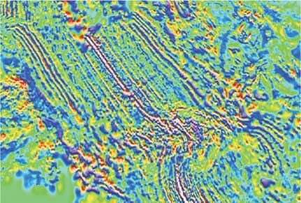
B02305                           WHITE AND SMITH: HATTON CONTINENTAL MARGIN                                           B02305

         Figure 1. Layout of normal incidence and wide-angle seismic profiles and ocean bottom seismometer
         locations (open circles) for the experiment reported here. Example record sections from OBS numbered
         and marked by crosses inside the circles are shown in Figures 3 and 4. HB89 is location of earlier wide-
         angle profile reported by Morgan et al. [1989] and shown in Figure 9b. Dotted profiles labeled A – H
         perpendicular to this show locations of expanding spread profiles used to constrain the dip line structure
         by White et al. [1987], Fowler et al. [1989], and Spence et al. [1989] and shown in Figure 9a. DSDP drill
         site 116 is shown by diamond. Filled circle at intersection of strike and dip lines shows location of
         vertical hydrophone array used to calculate air gun source waveform. Contours in meters, interval 200 m.

         Figure 2. Multichannel seismic reflection profile along dip line showing locations and numbering of
         OBSs and intersection point with main strike line. TB marks top basalt horizon, C30 and C10 mark
         regional unconformities in Hatton Basin that can be correlated with identical unconformities in Rockall
         Basin [Hitchen, 2004]. DSDP hole 116 [Laughton et al., 1972] is projected onto the profile from its
         location 11 km to the northeast (see Figure 1).

                                                          3 of 28
B02305                             WHITE AND SMITH: HATTON CONTINENTAL MARGIN                                             B02305

         Figure 3. Examples of vertical geophone recordings of wide-angle seismic data from the dip line: (a) OBS
         68, over oceanic crust in the Iceland Basin. (b) OBS 25, over continental crust of Hatton Bank (see Figures 1
         and 2 for location). Traces are scaled to a common maximum amplitude, band-pass-filtered 2 – 15 Hz, with
         traveltimes reduced at 7 km/s. Stars on inset show locations of OBS (see also Figures 1 and 2).

sediment velocities, we used semblance analysis on the             pick crustal diving phases Pg and Moho reflections PmP
coincident MCS profile, so they are unaffected by these            from almost all the OBS. This produced a data set of
errors.                                                            39,303 Pg and 10,008 PmP traveltimes on the dip and
  [10] No further processing was applied to the OBS data,          strike lines combined. Mantle refractions, Pn, were appar-
other than demeaning to remove a DC shift and application          ent on only some of the OBS (e.g., Figure 4b). In general,
of a 2 – 15 Hz zero-phase filter to attenuate noise. Examples      the arrivals were more consistent between adjacent OBS
of receiver gathers from two OBS on the dip line (Figure 3)        on the strike line with its limited lateral variability than on
and two on the strike line (Figure 4) demonstrate the quality      the dip line which crosses all the major structure created
of the arrivals. Plots of all the OBS receiver gathers are         during continental breakup. Uncertainties in the travel-
shown in the auxiliary material.1 Two OBS in the Maury             times were assessed for each arrival pick, according to the
Channel at the foot of the continental slope (Figure 2)            signal-to-noise ratio, varying in five steps from 20 ms for
were consistently noisier than other OBS, presumably due           the best arrivals to 120 ms for the poorest, where it was
to water currents, but other than those it was possible to         possible that the correct first arriving phase had been
                                                                   missed, resulting in a cycle skip. Reciprocity tests were
   1
     Auxiliary materials are available in the HTML. doi:10.1029/   made to check the consistency of traveltimes between pairs
2008JB005856.

                                                              4 of 28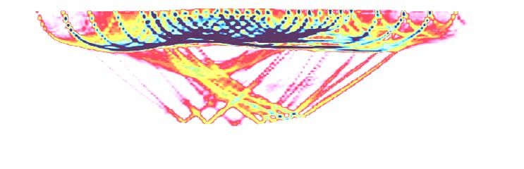
B02305                            WHITE AND SMITH: HATTON CONTINENTAL MARGIN                                          B02305

         Figure 4. Examples of vertical geophone recordings of wide-angle seismic data from strike line:
         (a) OBS 48, to the southwest. (b) OBS 38 to the northeast. Traces are scaled to a common maximum
         amplitude, band-pass-filtered 2 – 15 Hz, with traveltimes reduced at 7 km/s. Stars on inset show locations
         of OBS (see also Figure 1).

of shotpoints and OBSs [Zelt and Smith, 1992], and arrival       A variety of resolution tests were also constructed. In the
picks reassessed where there was a discrepancy of more           following description we use the dip line to explain the
than 150 ms.                                                     procedure.
                                                                   [12] The first stage was to use the velocimeter and XBT
4. Tomographic Traveltime Inversion                              measurements, together with the 10 kHz echo sounder
                                                                 records to constrain the water layer velocity structure and
  [11] We constrained the 2-D crustal velocity model by          thickness. The sediment layer seismic velocity and thick-
tomographic inversion of the traveltimes of the main P wave      ness was calculated from semblance analysis of the MCS
arrivals. This was done in four stages, each one using the       streamer data. In this area the sediments are thin (
B02305                            WHITE AND SMITH: HATTON CONTINENTAL MARGIN                                             B02305

defined by a uniform 0.1 km by 0.1 km grid. Inversion             64 ms (c2 = 1.5), comprising an RMS misfit of 62 ms for Pg
reduced the c2 value of the initial input model from >6 to        arrivals and 65 ms from PmP reflections. Compared to the
3.7, with a final RMS misfit of 109 ms. It was not possible       FAST starting velocities there is little change in the velocity
to achieve a better fit without introducing short-wavelength      structure of the upper crust, which is unsurprising since this
anomalies that were beyond the resolving power of the data        part of the model is constrained primarily by diving wave
set. The final model from this stage is shown in Figure 5a.       Pg arrivals. However, the lower crustal region has more
The upper 5 – 10 km of the crust is well constrained by           structure in the Tomo2D inversion than in the previous
crossing raypaths, but the deeper crust is only poorly con-       Rayinvr inversion, which again is consistent with the
strained by some deeper penetrating first arrival diving waves    Tomo2D grid parameterization which allows more detail
and a small number of Pn mantle refractions (Figure 5b).          to be modeled than does the single velocity gradient layer of
  [14] Since there are numerous strong wide-angle reflec-         the Rayinvr inversion.
tions off the Moho (PmP) with 7850 separate traveltimes on          [18] The Tomo2D model was defined by 59,274 velocity
the dip line, these were introduced in a third inversion step     nodes across a 400-km-long by 40-km-deep model domain.
using the forward ray-tracing modeling program Rayinvr            The node spacing was 0.5 km in the horizontal direction,
[Zelt and Smith, 1992]. The velocity structure down to 10 km      with the vertical node spacing increasing from 0.05 km near
depth constrained by the previous inversion step with FAST        the surface to 1 km at the base. The Moho reflector was
was held fixed. Since Rayinvr ray traces through a layered        defined by 401 modes with a uniform 1 km spacing. Since
model with interfaces, whereas the previous inversion with        we identified only a few unambiguous mantle refraction Pn
FAST used a regular grid of nodes, the Rayinvr model for the      phases, we did not attempt to invert structure beneath the
top 10 km was constructed by sampling the FAST velocity           Moho. Correlation lengths for the inversion are defined in
field over a 1.0 by 0.5 km grid with the rows of the grid         the horizontal and vertical directions as the dimensions of
forming the layers of the Rayinvr model. The boundaries of        the ellipse about which the inversion samples the model and
the rows were used to represent interfaces, with identical        attempts to fit the observed data [Korenaga et al., 2000], so
velocities above and below each interface to avoid artificial     they represent the minimum size of anomaly which may be
velocity discontinuities. The lower crust beneath 10 km and       resolved. This varies with depth. If the correlation lengths
extending down to the Moho was represented by a single            are too small, artifacts at a small scale may be introduced,
layer with a uniform vertical velocity gradient, which was        producing a rough model. We tested a range of different
allowed to vary laterally.                                        correlation lengths and chose values appropriate to the 9 Hz
  [15] The final best fit Rayinvr model had an RMS misfit         dominant frequency of the arrivals and the size of the
of 120 ms (c2 = 1.85), and successfully ray traced 98% of         Fresnel zone at the appropriate depth. The final inversions
the observed traveltimes (Figures 5c and 5d). We analyzed         used a horizontal correlation length which increased linearly
model uniqueness by testing 10 different starting models with     from 4 km at the seafloor, which is the minimum OBS
varying initial Moho depths and lower crustal velocities.         spacing, to 10 km at the base of the model. The vertical
These show that the lower crust is well constrained over the      correlation length increased from 0.2 km at the seafloor to
interval from 50 to 250 km along the model, particularly in       7 km at the base.
the region of primary interest straddling the COT, with little      [19] We used a 1 km correlation length for the Moho
variation from the different inversions in the velocities and     reflector to match the node spacing, which allows the trade-
Moho depths across this section of the profile. Standard          off between velocity and depth to be evaluated properly
errors from the Rayinvr covariance matrix are typically less      [Korenaga et al., 2000]. Tests of the velocity-depth trade-
than 0.07 km/s for velocity and 0.4 km for Moho depth across      off for the Moho reflector were made by repeating the
this well-constrained region.                                     inversions with varying weights applied to the crustal
  [16] Although the Rayinvr model provides a satisfactory         velocity and depth perturbation updates. The depth weight-
fit to the traveltime observations, it has several limitations,   ing kernel, w, was varied from w = 0.01 to test the model
chief among which is the user-defined parameterization of         generated when the inversion favored larger velocity and
the number and node spacing of interfaces, which may lead         smaller depth perturbations, through equal weighting with
to bias in the final model. Other limitations include mod-        w = 1, to the opposite relative weighting of depth and velocity
eling the lower crust as a single layer, which therefore limits   with w = 100. The fit to all three models is similar (see
resolution of detailed velocity variations within that layer,     Figure S1 in the auxiliary material), a consequence of the
other than those which can be expressed by a uniform              high number of crossing raypaths in the central part of the
vertical gradient, and the inversion of PmP reflections which     model between 50 and 250 km distance, so for the final
permit velocity-depth ambiguity in the Moho which could be        models we chose equal weighting of velocity and depth
resolved if diving waves in the lower crust were inverted         updates (w = 1) for the Moho reflector inversions.
simultaneously.
  [17] We therefore moved to a final tomographic inversion        4.1. Resolution Tests
technique, Tomo2D developed by Korenaga et al. [2000],              [20] Traveltime inversions are inherently nonunique, so
which jointly inverts refraction traveltimes through the          we spent considerable effort in assessing the resolution of
model as well as reflection traveltimes from a chosen single      the model. Since we had a dense data set, a simple test was
reflector, which in our case is the Moho. We used a total of      to split the data into two parts and to invert them separately
17,639 Pg arrivals and 7850 PmP arrivals in the dip line          to investigate the similarity of the two inversions. For this
inversion. Using a starting model derived from the previous       test we chose a simple starting model with a 1-D crustal
modeling steps, we derive the velocity distribution shown in      velocity structure hung beneath the base of the sediments
Figure 5e, which has an overall RMS traveltime misfit of          and a flat Moho at 18 km depth (see Figure S2a in the

                                                             6 of 28
B02305
7 of 28
WHITE AND SMITH: HATTON CONTINENTAL MARGIN
Figure 5. Final tomographic inversion models for the dip line showing the sequence in which successively better
inversions were developed: (a) FAST [Zelt and Barton, 1998], using only first arrivals from crustal refractions Pg, achieving
c2 = 3.7 and RMS misfit of 109 ms. (b) FAST ray hit count illustrating ray coverage limited mainly to the upper crust.
(c) Rayinvr [Zelt and Smith, 1992] forward ray-traced model using the FAST model as a starting point for the upper crust,
constrained by both crustal refractions Pg and mantle reflections PmP with c2 = 1.85 and RMS misfit of 120 ms. (d) Rayinvr
ray hit count showing constraints on different areas of the model. (e) Tomo2D [Korenaga et al., 2000] final model using results
from FAST and Rayinvr models in the starting model, with final c2 = 1.5 and RMS misfit of 64 ms. (f) Tomo2D derivative
weight sum (DWS) showing good constraints on the ray coverage through the crust beneath Hatton Bank, the COT, and the
B02305
oceanic crust but poorer constraint on the southeastern part of the profile at distances >250 km.B02305 WHITE AND SMITH: HATTON CONTINENTAL MARGIN B02305
Figure 6. Range of basement 1-D velocity profiles and Moho reflector depths used to generate the
starting models for Monte Carlo modeling: (a) dip line and (b) strike line.
auxiliary material). Two independent data sets were made [23] A wide range of starting velocity models was used
by dividing the OBS into two sets, each distributed along the for the 100 randomized inversions. In each case a 1-D
profile. The long-wavelength structures obtained by invert- velocity model was hung from beneath the sediments to
ing the two partial data sets separately are consistent with avoid introducing unnecessary prior information. Since we
each other, and with the inversion results using all the OBS were not inverting any mantle velocities, a maximum initial
along the profile (see Figure S2). Differences are local and velocity of 7.5 km/s was defined at the base of the model. A
small, demonstrating that the major structure is real and is not flat initial Moho reflection depth was input independently of
an inversion artifact. the velocity structure. On the dip line, with its large crustal
[21] We also conducted checkerboard tests by introducing thickness variations, the starting Moho depth was allowed
alternating regions of positive and negative anomalies onto to vary from 15 to 30 km (Figure 6a), whereas on the strike
the final model, and adding random Gaussian noise to the line with its more restricted variation in crustal thickness,
traveltimes. Full details are given in the auxiliary material the Moho depth was allowed to vary slightly less between
(Figure S3), but in summary, the locations of the velocity 17 and 27 km depth (Figure 6b), so as to sample well the
perturbations were recovered well in the inversion, partic- most likely values.
ularly in the upper crust, although the recovered amplitude [24] The observed traveltimes were also randomized
of the velocity anomalies were only of the order of 1 – 2% of before inversion so as to take account of the likely uncer-
the background velocity, compared to the input anomalies tainty in the arrival picks. Simply adding random offsets to
of 5%. This is normal in checkerboard tests of this type, and each individual pick does not reproduce the likely errors,
is a consequence of the imposed smoothing inherent in the since it has the effect of producing rough traveltimes with
inversion algorithms. For our purposes the most important considerable variation between adjacent picks, but an overall
conclusion is that the significant lateral changes in velocity average of zero. Following Zhang and Toksöz [1998], a more
structure to which we attach geological importance in this realistic implementation of the likely traveltime errors is to
paper are all well resolved on an appropriate scale. add both a randomized receiver error, which accounts for
[22] In order to assess the robustness of our velocity models uncertainties in the clock drift correction and in fine-scale
and the resolution and uncertainty of the velocities at every structure beneath the OBS which is below the resolution of
position, we used a Monte Carlo technique as an approxima- the inversion, and a traveltime gradient error which simulates
tion to a Bayesian inference method [Tarantola, 1987]. possible user bias in picking along a phase. In the 100 dif-
By appropriately randomizing both the starting velocity ferent inversions we applied a random Gaussian noise distri-
models and the traveltimes, multiple inversions allow an bution with s2 = 50 ms for the common receiver uncertainty,
estimate to be made of the posterior mean and covariance of and a random Gaussian distribution with s2 = 25 ms/km for
the solution, from which it is possible to determine the the traveltime gradient uncertainty of a picked phase.
variance of the solution at any point in the model, together [25] The average 2-D velocity structure of all the Monte
with the associated resolution [Zhang and Toksöz, 1998; Carlo inversions for each profile (which we consider to be
Korenaga et al., 2000]. We use the term ‘‘Monte Carlo the best representation of the velocity structure), plus the
ensemble’’ to describe the average model which, together standard deviation of the average at every point along the
with the standard deviation of the velocities and depths profile, is shown in Figures 7 and 8 for the dip and strike
illustrates the results from all the individual Monte Carlo lines, respectively. In both cases the final, ensemble average
inversions. In this study we made 100 Monte Carlo inver- models are strikingly similar to the results of the inversion
sions of each profile, using the same inversion parameters using the best estimate of the starting model from prior
as chosen for the best fit model described earlier. FAST and Rayinvr inversions (e.g., compare Figure 7 with
Figure 5e). The model standard deviation calculated from
8 of 28B02305 WHITE AND SMITH: HATTON CONTINENTAL MARGIN B02305
Figure 7. (a) Final dip line Monte Carlo average from 100 randomized starting models, with region of
ray coverage highlighted; bold contours every 0.5 km/s; fine contours every 0.1 km/s above 7.0 km/s.
(b) Derivative weight sum showing raypath coverage. (c) Model standard deviation with bold velocity
contours drawn every 0.1 km/s and fine velocity contours drawn every 0.05 km/s. Error bars on Moho
show standard deviation for resolution of depth to Moho.
all 100 Monte Carlo inversions shows that the velocities on Monte Carlo ensemble averaged model from all the OBS,
both profiles are constrained to better than 0.1 km/s across together with the raypaths for each calculated traveltime.
almost all the model, with the weakest constraint (reaching
0.2 km/s uncertainty) restricted to a small area near the base 4.2. Comparison With Other Velocity Models
of the crust at 130 km on the dip line where the ray of Hatton Margin
coverage is poorest. Unsurprisingly, the velocity constraints [27] There are now three independent wide-angle profiles
are also poorer at the ends of the models. The standard across the Hatton margin, each processed and modeled
deviation of the Moho reflector depth is mostly in the range separately using different methods. So they provide a
0.6 – 1.0 km across the central regions of the profiles, good opportunity to compare different methods of constrain-
consistent with the dominant wavelength at the base of ing the crustal structure of a similar part of the margin. In
the crust of 700 m. Figure 9 the crustal structures published for each of the
[26] In the auxiliary material, we show the observed three profiles are redrawn at the same scale and then aligned
traveltime picks and calculated traveltimes through the final along strike.
9 of 28B02305 WHITE AND SMITH: HATTON CONTINENTAL MARGIN B02305
Figure 8. (a) Final strike line Monte Carlo average from 100 randomized starting models, with region
of ray coverage highlighted; bold contours every 0.5 km/s; fine contours every 0.1 km/s above 7.0 km/s.
(b) Derivative weight sum showing raypath coverage. (c) Model standard deviation with bold velocity
contours drawn every 0.1 km/s and fine velocity contours every 0.05 km/s. Error bars on Moho show
standard deviation for resolution of depth to Moho.
[28] The first dip section [from White et al., 1987, Figure 9a] used to model the traveltimes, then the velocity structure
was compiled from a series of expanding spread profiles was refined using amplitudes modeled with Fuchs and
recorded using two ships, one with a multichannel streamer Muller’s [1971] full reflectivity synthetic seismogram
and the other firing either an air gun array or up to method. The individual one-dimensional velocity profiles
62 explosive shots spaced 1 km apart, ranging in size from from each expanding spread profile at the locations labeled
2.1 kg at near offsets to 100 kg at far offsets. The expanding A – H in Figure 9a were then interpolated and contoured to
spread profiles were orientated along strike of the margin so construct the downdip cross section.
as to minimize lateral variations in structure (dotted lines in [29] The second dip section [see Morgan et al., 1989,
Figure 1 show locations of profiles). The expanding spread Figure 9b] is located along the center points of the expanding
profiles had to be interpreted assuming a one dimensional spread profiles (labeled HB89 on Figure 1) but was controlled
velocity-depth variation, apart from corrections for the by four OBS (two at each end), and a variable-offset two-ship
known water and sediment thicknesses beneath each ship. profile. The energy sources were 105 explosive shots fired
Cerveny and Psencik’s [1979] ray-tracing program was every 1.5 km and recorded on both the OBS and the multi-
10 of 28B02305 WHITE AND SMITH: HATTON CONTINENTAL MARGIN B02305
Figure 9. Comparison of models at the same scale of the velocity structure along dip profiles across the
Hatton Bank rifted margin, aligned at the same position along strike. COT marks continent-ocean
transition. (a) Model from White et al. [1987], with details published by Fowler et al. [1989] and Spence
et al. [1989], and constructed by interpolation and contouring between one-dimensional velocity-depth
profiles from the midpoints of 8 expanding spread profiles (A– H) orientated along strike at the locations
marked along the top of the profile and by dotted lines in Figure 1. The expanding spread profiles used a
mixture of explosives and air guns as sources and were modeled using reflectivity synthetic seismograms.
(b) Model from Morgan et al. [1989] along the dip line marked HB89 in Figure 1 using a downdip two-
ship air gun profile with variable offsets plus wide-angle arrivals from four four-component ocean bottom
seismometers at locations marked by ellipses at the seafloor, using 105 explosive shots as sources. The
data were modeled using Maslov asymptotic ray theory. (c) Final dip line Monte Carlo average velocity
structure from this paper modeled using Tomo2D traveltime tomography of arrivals at four-component
ocean bottom seismometers marked by ellipses at seafloor.
channel streamer. The traveltime data were modeled using the lower crust were higher than normal, introducing a small
Maslov asymptotic ray theory [Chapman and Drummond, low-velocity zone between the extrusive lavas that produce
1982], which allows for two-dimensional structure. The seaward dipping reflectors on the COT and the underlying
starting model for the crustal velocity model was derived lower crust.
from the expanding spread profiles. Discontinuities were [30] The third dip section (Figure 9c from the Monte Carlo
introduced in the region of the COT where the velocities of average of the randomized Tomo2D inversions reported in
11 of 28B02305 WHITE AND SMITH: HATTON CONTINENTAL MARGIN B02305
this paper) is about 30 km along strike to the south of the weight sum and the standard deviation of all 100 inversions
previous two profiles (Figure 1). It was recorded using a large from randomized starting models (as shown in Figures 7b, 7c,
air gun source array and a dense array of four-component 8b, and 8c) give a good indication both of the areas of the
OBS as described in section 2. model that are constrained well by the data, and of how much
[31] Despite the different methodologies of both record- deviation in velocity structure is allowable in any particular
ing and interpreting the wide-angle data, the main features area of the model. By contrast it is difficult to gain any
of all three different profiles are consistent. They each show constraint on the possible range of velocity models from the
a relatively narrow transition from continental to oceanic interpolated 1-D models of Figure 9a. In the case of the
crust, and each one requires high-velocity material in the forward ray-traced model which produced Figure 9b, Morgan
lower crust of the COT. The actual crustal velocities inferred et al. [1989] gave no indication of the allowable range of
are similar in all three profiles (generally within 0.1 km/s). models but commented that it was hard to find a model which
The overall crustal thickness and its variation across the matched all the data. They report trying 700 different models
continental margin are also similar. It is certainly encour- before finding a satisfactory fit. In such circumstances, the
aging to have this degree of agreement in the main features ray coverage is perhaps the best indication of which parts of
that are used for interpretation. However, the more interest- the model are constrained, while checkerboard tests provide
ing question lies in the differences between the profiles. an indication of the magnitude and dimensions of velocity
These differences lie mainly in the resolution that the perturbations that could in principle be resolved.
different methods provide, and in the constraints that can [34] It is worth commenting that the models shown in
be placed on the uncertainties in the models. Figures 9a– 9c have been derived primarily from the travel-
[32] Not surprisingly, the resolution increases from the times of P waves. Clearly there is much more information
smoothest model in Figure 9a, interpolated from one-dimensional available in the seismic data than just the traveltimes. Where
velocity-depth profiles, through the variable-offset model in converted S waves are generated, then they can provide con-
Figure 9b to the model constrained by closely spaced OBS straints on the Poisson’s ratio of the rocks, which may help
in Figure 9c. Perhaps more importantly, the denser wide- with interpretation [e.g., Eccles et al., 2007]. The obvious
angle coverage provided by the multiple crossing raypaths next step is to use the amplitudes of the arrivals to refine the
from the closely spaced OBS array in the most recent profile velocity structure. Amplitudes are particularly sensitive to the
allows an automated tomographic inversion to be employed. sharpness of velocity changes and to velocity gradients.
This is better than the trial and error forward ray tracing Hitherto it has proven possible to use amplitude information
modeling used to construct Figure 9b because although that with the assumption of local 1-D structure, as Fowler et al.
model fits the arrival times within their estimated uncertain- [1989] demonstrated in deriving the structure shown in
ties, the sharp interfaces marked by the dotted lines have been Figure 9a. As computer processing power has increased, it
inserted by the modeler. Although at first sight they may has become realistic to derive acoustic waveform inversion
appear to indicate high-resolution control on the discontinu- constraints provided the models are limited in size and
ities, in practice they are only one possibility from an infinite contain good low-frequency content to constrain the lon-
number. Indeed, geologically, it is unlikely that such sharp ger-wavelength structure [e.g., Brenders and Pratt, 2007]. At
subvertical discontinuities exist in highly stretched and present, the computing power that would be required means
heavily intruded crust. In contrast, the average structure that it is not realistic to make full elastic inversions of whole
from 100 inversions with randomized starting models crustal models similar to those shown here from the Hatton
shown in Figure 9c shows a better depiction of the structure margin, but doubtless it will be in due course. The expectation
that can be constrained unambiguously by the data. It is is that the long-wavelength structure shown in Figures 7 – 9
theoretically possible that the true structure contains sharp would not change, but the constraints on local discontinuities
subvertical discontinuities within it, but that the multiple and velocity gradients would improve, giving better resolution.
inversions mask that solution – if so, that is a helpful result,
because it means that the data do not require a sharp 5. Interpretation
discontinuity, so we could not put prominence on one in
our interpretation. However, a corollary to this statement is [35] In the following sections we discuss in turn the main
that sometimes the profile does indeed contain sharp dis- tectonic provinces crossed by the dip line profile. At the
continuities that we do know about, such as the seafloor continentward (southeastern) end the profile crosses the
interface and the sediment-basement interface. If we did not Mesozoic Hatton Basin followed toward the northwest by
force the inversion to introduce these interfaces, then it the Hatton Bank continental block, then the COT with its
would produce smoothed velocity changes across them, characteristic seaward dipping reflectors in the upper crust
with the smoothness controlled mainly by the grid size of and finally oceanic crust with seafloor spreading magnetic
the inversion. In the inversion modeling it is normal to anomalies.
introduce a sharp discontinuity at the seafloor and to heavily 5.1. Hatton Basin
damp the structure, such as sediment thickness that is
known independently (for example from seismic reflection [36] The Hatton Basin is the least constrained portion of the
profiles). profile, due to the sparse OBS spacing. Nevertheless, good
[33] Perhaps more significantly, the newer and denser data wide-angle Moho reflections were recorded, constraining the
sets enable an objective measure of the uncertainty in the crustal thickness as 19–21 km, with a Moho depth uncer-
velocities and depths to be placed on the inversion models as tainty of 1 km. The basin was formed by Mesozoic
well as using them to define a ‘‘best’’ average model. The stretching before the Tertiary continental breakup. Our dip
combination of ray densities as measured by the derivative profile (Figure 2) crosses the flank of the late Paleocene
12 of 28B02305 WHITE AND SMITH: HATTON CONTINENTAL MARGIN B02305
Figure 10. (a) Comparison of the average crustal velocity structure in Hatton Basin (averaged from
240 to 310 km along iSIMM dip profile) with the structure beneath Hatton Basin 55 km to the SW
(CDP87-3 [Keser Neish, 1993]) and 200 km to the SW (RAPIDS V98 [Vogt et al., 1998]). (b) Comparison
of Hatton Bank velocity structure at 180 km along dip profile with the structure beneath Rockall Bank
(B79 [Bunch, 1979]) and Ireland (COOLE 85-1 [Landes et al., 2005]). (c) Velocity structure of the
continent-ocean transition at 150 km along dip profile, with comparison curves from continental crust at
180 km and oceanic crust at 120 km along profile. (d) Velocity structure of oceanic crust at 120 km along dip
profile compared to normal oceanic crust (gray shading, all Atlantic oceanic profiles away from fracture
zones and plumes from White et al. [1992]). The iSIMM velocity profiles are constrained to the base of the
crust only, so an appropriate velocity contrast has been added to indicate the position of the Moho. Note that
curves in Figures 10a and 10b show depth below sea level, while curves in Figures 10c and 10d show depth
below the top of the basement.
Lyonesse igneous complex, with extrusive lavas covered by a some 55 km to the southwest by Keser Neish [1993] and
thin veneer of Cenozoic sediments [Hitchen, 2004]. The from the RAPIDS profile about 200 km away by Vogt et al.
Hatton Basin was submarine at the time of continental [1998] (see Figure 10a). If we assume that the crystalline
breakup, with the western paleoshoreline marked by a steep basement thickness before stretching was 28 km, as sug-
basalt escarpment (at 310 km on Figure 2). Eocene fan deltas gested by the nearest wide-angle seismic profiles on Rockall
formed at the base of this scarp [McInroy et al., 2006], and the Bank [Bunch, 1979] and in Ireland [Landes et al., 2005],
Hatton Basin was filled subsequently by ~2 km of Cenozoic then we infer a Mesozoic stretching factor of 2.2 ± 0.3 in
sediment. Hatton Basin (Table 1). This is considerably less than the
[37] The crustal thicknesses we deduce for the Hatton probably contemporaneous stretching in nearby Rockall
Basin are similar to those reported from profile CDP87-3 Trough to the east [Joppen and White, 1990].
13 of 28B02305 WHITE AND SMITH: HATTON CONTINENTAL MARGIN B02305
Table 1. Stretching Factors Across Rockall Plateaua
Source Depth to Moho (km) Crustal Thickness (km) Stretching Factor
Ireland Landes et al. [2005] 29.8 – 31.8 ± 1 28 ± 1 1.0
Rockall Bank Bunch [1979] 29.8 – 31.0 ± 1 28 ± 1 1.0
Hatton Basin iSIMM, this paper 20.4 ± 0.90 12.5 ± 1.1 2.24 ± 0.3
Hatton Bank iSIMM, this paper 24.8 ± 0.55 22.5 ± 0.75 1.24 ± 0.1
a
The thickness under Ireland and Rockall Bank is used as prestretching reference thickness. The Moho beneath both Ireland and Rockall was interpreted
as a transition zone. Uncertainties in the depth to Moho and crustal thickness for both Ireland and Rockall were estimated to be ±1 km. Uncertainties in
crustal thickness along the iSIMM line take into account both the error in depth to Moho and error in identifying the top of the crystalline basement.
5.2. Hatton Bank [42] The seismic profile modeled here spans 120 km of
[38] Hatton Bank is a block of continental crust with a oceanic crust along the dip profile, which covers the first
maximum thickness of 23 km between the Hatton Basin 8 Ma of seafloor spreading following breakup at 54 Ma.
on the east and the COT on the west. It has a thin There is a consistent pattern as the crust becomes younger
veneer of Cenozoic sediments, only 50 m thick in the of a decreasing thickness and a concomitant decrease in the
shallowest portion. The Cenozoic sediments are underlain average velocity of the lower crust, with the highest velocity
by a 1.2 km thick layer with a steep velocity gradient found in the oldest and thickest oceanic crust adjacent to the
from 4.7 km/s at the top to 5.5– 5.9 km/s at the base COT. A similar result has been reported by Parkin and
(Figure 10b). Seismic profiles and shallow drilling in the White [2008], who independently modeled just the oceanic
area shows that Hatton Bank is covered by a layer of section of this profile, and extended it out to younger
extruded basalts, but that in places they have been eroded oceanic crust generated at 39 Ma. The oceanic crust is
to expose underlying Mesozoic and possibly Paleozoic everywhere thicker than the normal segment-averaged
sediments [Hitchen, 2004]. crustal thickness of 6.4 ± 0.8 km [White et al., 1992; Bown
[39] The bulk of the crust beneath the thin sedimentary and White, 1994]. Weak gravity lineations at 48 Ma and
and basalt section comprises material with a low velocity 39 Ma visible on both sides of the ocean basin may be
gradient from 5.5 to 5.9 km/s at the top to 6.94 ± 0.06 km/s caused by small crustal thickness increases similar to those
at the base (Figure 10b). This is typical of the crystalline that produce the V-shaped ridges on the young crust of this
crust found beneath the adjacent Rockall Bank continental ocean basin [Parkin and White, 2008], but they are beyond
fragment [Bunch, 1979] and the closest continental main- the extent of the profile we report here.
land beneath Ireland [Lowe and Jacob, 1989; Landes et al.,
2005], although it is here some 5 km thinner than beneath 5.5. Continent-Ocean Transition: Upper Crust
the mainland. From this we deduce that Hatton Bank has and Extrusive Basalts
been stretched by a factor of 1.2 ± 0.1 (Table 1). [43] The extrusive basalts on the COT form a series of
seaward dipping reflectors (SDRs). On dip profiles they often
5.3. Continent-Ocean Transition
exhibit a characteristic convex upward shape, as a result of
[40] The transition from the continental crust of Hatton crustal stretching and subsidence contemporaneous with
Bank to the oldest fully oceanic crust with well-developed their emplacement [Mutter et al., 1982]. Although their
seafloor spreading magnetic anomalies is extremely narrow, present dip is seaward, the lava was emplaced by landward
only some 40 km wide (between 130 and 170 km along the directed flow from a subaerial rift. The basalt sequence
dip profile, Figure 7a). Velocities in the lower crust of the reaches at least 5 km at its thickest on the COT and thins to
COT are intermediate between those of the adjacent conti- 1.5 km over the shallowest part of Hatton Bank. Similar
nental Hatton Bank on the east and the oceanic crust on the SDR sequences are found along all the North Atlantic
west (Figure 10c). White et al. [2008] showed that a volcanic margins [e.g., Larsen and Jakobsdottir, 1988;
similarly narrow COT has been found north of the Faroes Barton and White, 1997b; Holbrook et al., 2001].
and that the velocity cross section of both the Faroes and [44] In Figure 11 we show a compilation of interpreta-
Hatton COTs are remarkably similar. However, this is in tions of the upper crustal structure that shows the SDR
marked contrast to the reported 150-km-wide zone of tran- morphology from a grid of MCS profiles around the
sitional crust on the conjugate Greenland margin [Korenaga iSIMM lines reported here. Figures 11b and 11c are from
et al., 2000, 2002; Hopper et al., 2003]. We shall return later strike profiles and Figures 11d – 11h from dip profiles:
to the asymmetry of the conjugate margin and possible rea- Figures 11b, 11d, and 11e are redrawn at the same scale
sons for it. from sources listed in Figure 11 caption, while the others
are new interpretations either from the iSIMM cruise
5.4. Oceanic Crust
reported here or from the 1985 Hatton Bank cruise [White
[41] The oldest oceanic crust immediately adjacent to the et al., 1987]. Comparison with our wide-angle velocity
COT is identified by seafloor spreading magnetic anomaly tomography shows that below a carapace of thin Cenozoic
24 at the foot of the continental slope near the termination of sediments the seismic velocity of the layered basalts exhibit
the arcuate SDRs. It exhibits a classic oceanic crustal a high velocity gradient, with velocities increasing from
structure, an uppermost layer 2 with a high-velocity gradient 3.5 km/s at the top of the sequence to 5.5–6.5 km/s at the
underlain by a lower velocity gradient layer 3 down to the base. We interpret the velocity gradient through the basalts
Moho. The transition between layers 2 and 3 occurs at a as caused mainly by the increase in pressure with depth and
velocity of about 6.7 km/s (Figure 10d). the concomitant closure in fractures and pore space and in
14 of 28B02305 WHITE AND SMITH: HATTON CONTINENTAL MARGIN B02305
Figure 11
15 of 28B02305 WHITE AND SMITH: HATTON CONTINENTAL MARGIN B02305
part from filling of pore space by secondary minerals and a ductile conditions that allowed large amounts of crustal
reduction in alteration with depth. extension without brittle faulting.
[45] There are two main packages of SDRs on most of
the Hatton continental margin, imaged best on profile NI8 5.6. Continent-Ocean Transition: Lower Crust
(Figure 11e), but also evident on the other dip lines. The [49] The crustal thickness decreases rapidly across the
upper set of SDRs are thinner and more planar than the COT, from 23 km to 18 km over the 40 km interval from
lower set which span the COT. The planar geometry of the 170 to 130 km distance (Figure 12). The lower crust over
upper set suggests that they were emplaced onto continen- this same interval exhibits high seismic velocities, interme-
tal crust with greater flexural strength and less extension diate between the velocities of the continental Hatton Bank
than those on the highly extended and intruded COT, crust on the landward side and the higher velocities of the
which exhibit pronounced convex-up curvature. The two oceanic crust of the Iceland Basin on the seaward side
packages are separated on profile NI8 (Figure 11e) by a (Figures 10c). The high velocities are indicative of the
seismically opaque region extending from 140 to 155 km presence of igneous rocks in the lower crust, and are much
which could be either a continental fault block or an higher than found in the continental crust of NW Europe
igneous intrusion. On the Edoras Bank margin to the that is not affected by Tertiary igneous activity [White et al.,
south, a similar geometry was interpreted as a fault block, 1987]. There is some indication that the high-velocity rocks
with lavas ponding against it on the landward side [Barton extend a short distance landward beneath Hatton Bank at the
and White, 1997a, 1987b]. However, the limited lateral very base of the crust (Figure 7a), but such lateral intrusion
extent, high density and magnetization of the feature on is apparently limited, with the majority remaining beneath the
the Hatton margin led White et al. [1987], Spence et al. region of igneous extrusion marked by the seaward dipping
[1989], and Morgan et al. [1989] to interpret it as an reflectors on the COT.
igneous center. [50] Although our MCS profiles on the Hatton margin do
[46] On strike lines the SDRs are imaged as subhori- not image the lower crust, on another iSIMM profile north
zontal reflectors (Figures 11b and 11c), consistent with the of the Faroe Islands, a deep penetration MCS profile shows
basalts having been extruded from fissure swarms aligned that a similar narrow zone of elevated (>7.0 km/s) velocities
parallel to the rift. The thickness of the reflective basalts in the lower crust of the COT is coincident with extensive
varies along strike, as they flowed to fill lows in the lower crustal reflections interpreted as sills [White et al.,
topography. 2008]. Using the insights from the Faroes profile reported by
[47] Immediately beneath the basalt sequence on the White et al. [2008], we therefore interpret the lower crustal
COT, the crustal velocity is >6.5 km/s. This is higher velocities on the Hatton profile as representing a mixture of
than the velocity at the same depth beneath the continental igneous intrusives produced during continental breakup and
block of Hatton Bank, although we expect the rocks to be the residual continental crust on the COT into which they are
the same. The reason is probably that on the COT there intruded.
are sills and feeder dykes intruded into the consolidated [51] In Figure 12 we show the way in which the average
sediments that form the upper part of the prebreakup velocity of the lower crust increases across the COT along the
continental crust, and these raise the crustal seismic Hatton dip profile. It shows an increase of 0.59 ± 0.17 km/s
velocity. A similar effect, also attributed to igneous intru- from continental to oceanic crust with the maximum velocity
sions has been reported from the Ethiopian rift, where being reached as the first (oldest) oceanic crust of the Iceland
there is an abrupt increase from typical continental crustal Basin is formed. There is excellent agreement of the velocity of
velocities to crust with P wave velocities that are 5 – 10% the lower crust between the dip and strike profiles at the
higher (>6.5 km/s) in the region of the Boset volcanic rift intersection point, although they were modeled independently.
[Mackenzie et al., 2005]. 5.7. Melt Generation
[48] A striking characteristic of the upper crust of the
COT, in addition to its narrowness, is the absence of crustal [52] A key question is what causes the generation of huge
fault blocks such as are typically found on nonvolcanic quantities of igneous rock on volcanic rifted continental
margins, and indeed are inferred to be present on the margins such as this one. The suggestion that the main
conjugate east Greenland margin based on ODP drilling mechanism was decompression melting as hotter than
and high-resolution seismic profiles [Larsen and Saunders, normal mantle rose beneath a lithospheric rift was first
1998]. It is likely that initial fault blocks were obliterated by made by White et al. [1987] to explain the seismic high-
continued heavy igneous activity in the narrow band of the velocity lower crust mapped from seismic data from this
COT, or that the intrusion of melts at 1300°C, well above same Hatton continental margin; a similar suggestion to
the melting point of the shallow continental crust, created explain melting during stretching of the nonvolcanic Biscay
Figure 11. Line drawings of unmigrated time sections from MCS reflection profiles recorded by the 1985 Hatton and the
2002 iSIMM surveys across the Hatton margin. (a) Location map, with circles showing positions of OBS on iSIMM
profiles. (b) Strike line NI3 from White et al. [1987] using same distance scale as Figure 11c. (c) Strike line from iSIMM
survey reported here. (d) Dip line SAP1 from White et al. [1987]. (e) Dip line NI8 from Spence et al. [1989] showing
crossing of igneous center discussed in text. (f and g) Dip lines newly interpreted from original profiles. (h) Dip line iSIMM
L8 processed by N. Hurst (personal communication, 2007) and newly interpreted. Dip lines are all aligned on intersection
with iSIMM strike profile at 150 km distance along dip line scale.
16 of 28B02305 WHITE AND SMITH: HATTON CONTINENTAL MARGIN B02305
Figure 12. (a) Velocity structure from average of Monte Carlo tomographic inversions along dip line
(from Figure 8), with main interpretation of crustal types superimposed. (b) Mean lower crustal velocities
along the dip profile calculated across horizontal windows of 10 km. Open diamonds are calculated for an
11 km thick section above the Moho, with large open circle the average for the intersecting strike profile
between 70 and 110 km along the strike line. Black diamonds indicate lower crustal velocities from
oceanic crust calculated for the crust with velocities > 6.7 km/s (which represents layer 3 section least
affected by the changes in porosity and alteration that exert a strong control on the shallower, layer 2
velocities).
continental margin above mantle of normal temperature had of a water rich layer allowing additional melting because the
been made earlier by Foucher et al. [1982]. Several recent wet solidus is at a much lower temperature than the dry
models have suggested that a mantle thermal anomaly is solidus, but again they could not get a large volume of melt
required to explain the excess magmatism on volcanic produced in their models because little melt was produced
margins, sometimes also with small-scale convection [e.g., before the mantle dehydrated and returned to the dry solidus
Nielsen and Hopper, 2002, 2004]. More recently, alternative and a much higher viscosity.
suggestions to explain the melting on volcanic margins have [53] We will not repeat here a discussion of the broader
included small-scale convection under the rift without a evidence that may be used to test the mantle plume theory
significant temperature anomaly in the mantle, or the for melt generation on volcanic rifted margins, since that
presence of fertile mantle beneath the rift which therefore has been reviewed recently by Campbell [2007] and by
was more readily melted [e.g., Mutter and Zehnder, 1988; others in numerous articles on different volcanic margins.
Korenaga et al., 2000, 2002]. We note, however, that the Instead we use the new constraints on the seismic velocity
fertile mantle source normally invoked is an iron rich layer, and thickness of the igneous crust on the margin to address
but Nielsen and Hopper [2004] showed that the high the narrower question of whether it can be explained
density of such a layer would prevent it from convecting. adequately by the presence of a thermal anomaly in the
Nielsen and Hopper [2004] also investigated the possibility mantle during rifting, or whether either the occurrence of
17 of 28You can also read