Hydraulic shortcuts increase the connectivity of arable land areas to surface waters
←
→
Page content transcription
If your browser does not render page correctly, please read the page content below
Hydrol. Earth Syst. Sci., 25, 1727–1746, 2021
https://doi.org/10.5194/hess-25-1727-2021
© Author(s) 2021. This work is distributed under
the Creative Commons Attribution 4.0 License.

Hydraulic shortcuts increase the connectivity
of arable land areas to surface waters
Urs Schönenberger and Christian Stamm
Eawag, Swiss Federal Institute of Aquatic Science and Technology, 8600 Dübendorf, Switzerland

Correspondence: Christian Stamm (christian.stamm@eawag.ch)

Received: 29 July 2020 – Discussion started: 7 September 2020
Revised: 22 February 2021 – Accepted: 1 March 2021 – Published: 6 April 2021

Abstract. Surface runoff represents a major pathway for pes-          servations led to shifts in estimated fractions of connected
ticide transport from agricultural areas to surface waters.           areas compared to the previous connectivity model. The dif-
The influence of artificial structures (e.g. roads, hedges, and       ferences were most pronounced in flat areas of river valleys.
ditches) on surface runoff connectivity has been shown in                These numbers suggest that transport through hydraulic
various studies. In Switzerland, so-called hydraulic short-           shortcuts is an important pesticide flow path in a landscape
cuts (e.g. inlet and maintenance shafts of road or field storm        where many engineered structures exist to drain excess wa-
drainage systems) have been shown to influence surface                ter from fields and roads. However, this transport process is
runoff connectivity and related pesticide transport. Their oc-        currently not considered in Swiss pesticide legislation and
currence and their influence on surface runoff and pesticide          authorization. Therefore, current regulations may fall short
connectivity have, however, not been studied systematically.          in addressing the full extent of the pesticide problem. How-
    To address that deficit, we randomly selected 20 study ar-        ever, independent measurements of water flow and pesticide
eas (average size of 3.5 km2 ) throughout the Swiss plateau,          transport to quantify the contribution of shortcuts and val-
representing arable cropping systems. We assessed short-              idating the model results are lacking. Overall, the findings
cut occurrence in these study areas using three mapping               highlight the relevance of better understanding the connec-
methods, namely field mapping, drainage plans, and high-              tivity between fields and receiving waters and the underlying
resolution aerial images. Surface runoff connectivity in the          factors and physical structures in the landscape.
study areas was analysed using a 2 × 2 m digital elevation
model and a multiple-flow algorithm. Parameter uncertainty
affecting this analysis was addressed by a Monte Carlo sim-
ulation. With our approach, agricultural areas were divided           1   Introduction
into areas that are either directly, indirectly (i.e. via hydraulic
shortcuts), or not at all connected to surface waters. Finally,       Agriculture has been shown to be a major source for pes-
the results of this connectivity analysis were scaled up to the       ticide contamination of surface waters (Stehle and Schulz,
national level, using a regression model based on topographic         2015; Loague et al., 1998). Pesticides are known to pose a
descriptors, and were then compared to an existing national           risk to aquatic organisms and to cause biodiversity losses
connectivity model.                                                   in aquatic ecosystems (Malaj et al., 2014; Beketov et al.,
    Inlet shafts of the road storm drainage system were iden-         2013). To implement effective measures to protect surface
tified as the main shortcuts. On average, we found 0.84 in-           waters from pesticide contamination, the relevant transport
let shafts and a total of 2.0 shafts per hectare of agricultural      processes have to be understood.
land. In the study catchments, between 43 % and 74 % of the              Pesticides are lost to surface waters through various path-
agricultural area is connected to surface waters via hydraulic        ways from either point sources or diffuse sources. In cur-
shortcuts. On the national level, this fraction is similar and        rent research, surface runoff (Holvoet et al., 2007; Larsbo et
lies between 47 % and 60 %. Considering our empirical ob-             al., 2016; Lefrancq et al., 2017), preferential flow through
                                                                      macropores into the tile drainage system (Accinelli et al.,

Published by Copernicus Publications on behalf of the European Geosciences Union.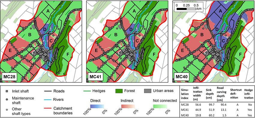
1728                   U. Schönenberger and C. Stamm: Hydraulic shortcuts connect arable land areas to surface waters

2002; Leu et al., 2004a; Reichenberger et al., 2007; Sandin et      ment lost to surface waters was transported through short-
al., 2018), and spray drift (Carlsen et al., 2006; Schulz, 2001;    cuts.
Vischetti et al., 2008) are considered of major importance.            To our knowledge, these two studies are the only ones
Other diffuse pathways, like leaching into groundwater and          systematically assessing the occurrence of hydraulic short-
exfiltration into surface waters, atmospheric deposition, or        cuts and their influence on (sediment) connectivity. However,
aeolian deposition, are usually less important.                     since these studies only covered a small total area in specific
   Past research showed that different catchment parts can          regions, it remains unknown if these findings are generally
largely differ in their contribution to the overall pollution of    valid for Swiss agricultural areas.
surface waters (Pionke et al., 1995; Leu et al., 2004b; Go-            Furthermore, two other studies in Switzerland addressed
mides Freitas et al., 2008). This is the case for soil erosion or   connectivity on a larger scale using a modelling approach.
phosphorus and also for pesticides. Areas largely contribut-        Both indicated that more areas were connected through
ing to the overall pollution load are called critical source        shortcuts than being directly connected. Bug and Mosimann
areas (CSAs). Models delineating such CSAs assume that              (2011) estimated 12.5 % of the arable land in the canton of
those areas fulfil the following three conditions (Doppler et       Basel-Landschaft to be directly connected to surface wa-
al., 2012): (i) they represent a substance source (e.g. pesti-      ters and 35 % to be connected indirectly. Later, Alder et
cides, soil, or phosphorus), (ii) they are connected to surface     al. (2015) created a national connectivity map of erosion
waters, and (iii) they are hydrologically active (e.g. formation    risk areas. They estimated that 21 % of the agricultural area
of surface runoff).                                                 is connected directly to surface waters and 34 % indirectly.
   Linear landscape structures, such as hedges, ditches, tile       Since the occurrence of hydraulic shortcuts was effectively
drains, or roads, have been shown to be important features for      known for small areas only, generalizing assumptions were
the connectivity within a catchment (Fiener et al., 2011; Rü-       made in both studies on the occurrence of hydraulic short-
bel, 1999). Undrained roads were reported to intercept flow         cuts (e.g. classification of roads as drained by shortcuts or
paths, to concentrate and accelerate runoff, and, therefore,        as undrained, based on their size). As also stated by Alder
also to influence pesticide connectivity within a catchment         et al. (2015), these assumptions are a major source of uncer-
(Carluer and De Marsily, 2004; Dehotin et al., 2015; Heath-         tainty. Their influence on the estimated connectivity fractions
waite et al., 2005; Payraudeau et al., 2009). Additionally,         remains unclear.
Lefrancq et al. (2013) showed that undrained roads act as              In summary, previous studies on hydraulic shortcuts were
interceptor of spray drift, possibly leading to significant pes-    either restricted to small study areas in a specific region or
ticide transport during subsequent rainfall events when inter-      were based on generalizing assumptions, lacking a spatially
cepted pesticides are washed off the roads.                         explicit consideration of hydraulic shortcuts. This study aims
   However, such linear structures and the related connectiv-       to present a systematic, spatially distributed, and represen-
ity effects exhibit substantial regional differences due to nat-    tative assessment of hydraulic shortcut occurrence on Swiss
ural conditions or various aspects of the farming systems.          agricultural areas. Based on this assessment, we aim to quan-
In contrast to other countries, many roads in agricultural ar-      tify the influence of hydraulic shortcuts on surface runoff
eas in Switzerland are drained by storm water drainage sys-         connectivity and pesticide transport. Additionally, we aim to
tems (Alder et al., 2015). Inlet shafts of such systems are         estimate how additional data on the occurrence of shortcuts
also found directly in fields (Doppler et al., 2012; Prasuhn        influence the connectivity fractions reported by the existing
and Grünig, 2001). Since they were reported to shortcut sur-        national connectivity map. We focused our study on arable
face runoff to surface waters, those structures were called         land, since this is the largest type of agricultural land with
hydraulic shortcuts or short circuits. Doppler et al. (2012)        common pesticide application in Switzerland.
showed that, in a small Swiss agricultural catchment, hy-              Our research questions, therefore, are as follows:
draulic shortcuts connected remote areas to surface waters
and had a strong influence on pesticide transport. Only 4.4 %        1. How widespread is the occurrence of hydraulic short-
of the catchment area was connected directly to surface wa-             cuts in Swiss arable land areas?
ters, while 23 % was connected indirectly (i.e. via hydraulic
                                                                     2. What is the contribution of hydraulic shortcuts to sur-
shortcuts). For the same catchment, Ammann et al. (2020)
                                                                        face runoff connectivity, and what are potential impli-
showed that the uncertainty of a pesticide transport model
                                                                        cations for surface-runoff-related pesticide transport?
could be reduced by 30 % by including catchment-specific
knowledge about hydraulic shortcuts and tile drainages.              3. How do additional data on the occurrence of shortcuts
   The occurrence of hydraulic shortcuts and their influence            influence the connectivity predictions at the national
on catchment connectivity has only been studied for a few               scale?
other catchments in Switzerland. Prasuhn and Grünig (2001)
found that only 3.2 % of the arable land in five small catch-
ments was connected directly to surface waters, while 62 %
was connected indirectly. Consequently, 90 % of the sedi-

Hydrol. Earth Syst. Sci., 25, 1727–1746, 2021                                        https://doi.org/10.5194/hess-25-1727-2021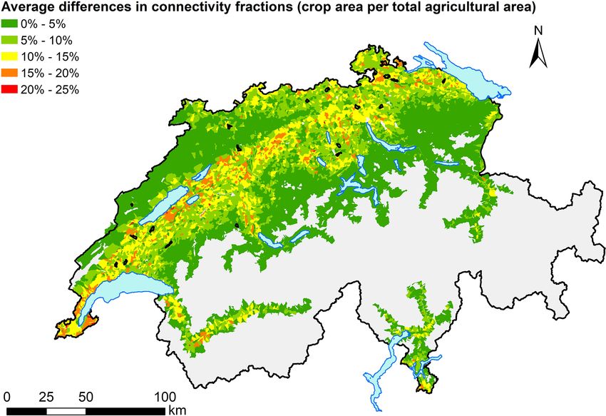
U. Schönenberger and C. Stamm: Hydraulic shortcuts connect arable land areas to surface waters 1729
b. maintenance shafts of storm drainage systems or tile
drainage system on roads, farm tracks, and crop areas;
and
c. channel drains and ditches on roads, farm tracks, and
crop areas.
If one of these structures is present, we defined this as a po-
tential shortcut. If surface runoff can enter the structure and
if the structure is drained to surface waters or to a wastewater
treatment plant, this is defined as a real shortcut. Other pro-
cesses that are sometimes referred to as hydraulic shortcuts
(e.g. tile drains) are not considered in this study. Tile drains
have already received considerable attention in pesticide re-
search and the transport to tile drains includes flow through
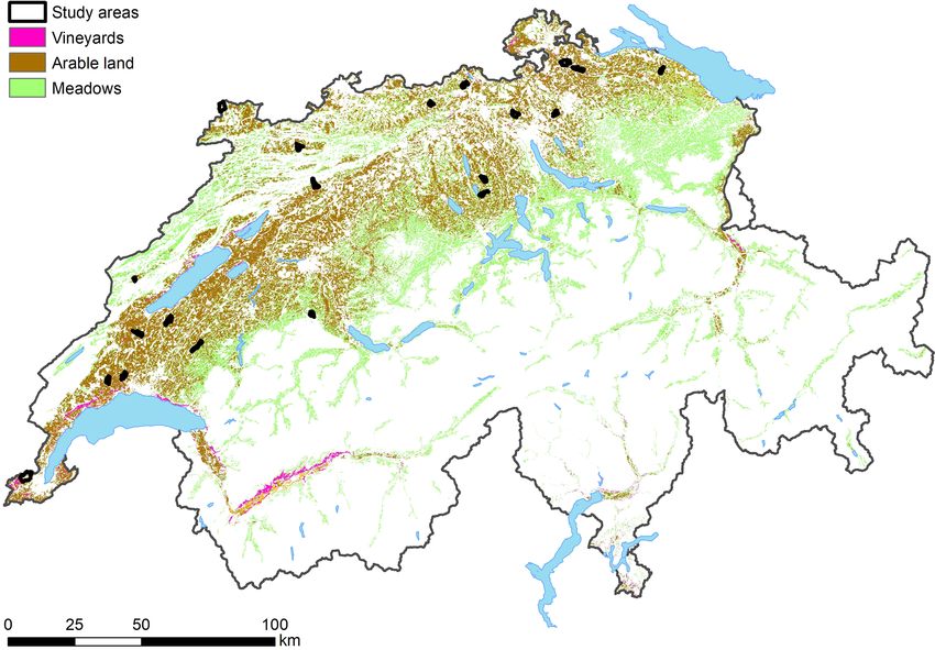
Figure 1. Study areas (black) and distribution of arable land natural soil.
(brown), vineyards (pink), and meadows and/or pastures (green)
across Switzerland. Sources: Swisstopo (2010); BFS (2014). 2.2.2 Shortcut location and type
We mapped the location and types of potential shortcuts in
2 Material and methods each study area by combining three different methods.
2.1 Selection of study areas i. Field survey. Field surveys were performed between
August 2017 and May 2018 (for details, see Table S5).
We selected 20 study areas (Table 1) representing arable land In a subpart of each study area, we walked along roads
in the Swiss plateau and the Jura mountains (Fig. 1). This and paths and mapped all the potential shortcut struc-
selection was performed randomly on a nationwide, small- tures. The starting point was selected randomly, and we
scale topographical catchment data set (BAFU, 2012). The mapped as much as we could within 1 d. Consequently,
probability of selection was proportional to the total area of the field survey data only cover part of the catchment.
arable land in the catchment, as defined by the Swiss land use For each of the potential shortcuts, we recorded its lo-
statistics (BFS, 2014). Random selection was performed, us- cation and a set of properties using a smartphone and
ing the pseudo-random number generator Mersenne Twister the application called Google My Maps. This included a
(Matsumoto and Nishimura, 1998). specification of the type of the shortcut (e.g. inlet shaft,
On average, the study areas have a size of 3.5 km2 and maintenance shaft, ditch, or channel drain), its lid type
are covered by 59 % agricultural land. The agricultural land (e.g. grid, sealed lid, or a lid with small openings), and
mainly consists of arable land (74 %) and meadows and/or its lid height relative to the ground surface. A list of
pastures (21 %). The mean slope on agricultural land is 4.9◦ , all possible types can be found in the Supplement (Ta-
and the mean annual precipitation amounts to 1159 mm yr−1 . bles S2 to S4).
A comparison of important catchment properties of the study ii. Drainage plans. For all municipalities covering more
areas to the corresponding distribution of all Swiss catch- than 5 % of a study area, we asked the responsible
ments with arable land demonstrated that the study areas rep- authorities to provide us with their plans of the road
resent the national conditions well (see Fig. S1). storm drainage systems and the agricultural drainage
systems. For 38 and 26 of the 46 municipalities con-
2.2 Assessment of hydraulic shortcuts
cerned, we received road storm drainage system plans
2.2.1 Shortcut definition and tile drainage system plans, respectively. Reasons
for missing data are either that the responsible authori-
We define a hydraulic shortcut as an artificial structure in- ties did not respond or that data on the drainage systems
creasing and/or accelerating the process of surface runoff were not available. From the plans, we extracted the lo-
reaching surface waters (i.e. rivers, streams, and lakes) or cations of shortcuts, and if available, the same proper-
making this process possible in the first place. In this ties were specified as in the field survey.
study, we focused on the following structures (example pho-
iii. Aerial images. Between August 2017 and August 2018
tographs can be found in Figs. S2 to S13):
(see Table S5), we acquired aerial images of the study
a. storm drainage inlet shafts on roads, farm tracks, and areas with a ground resolution of 2.5 to 5 cm. We used
crop areas; a fixed wing UAV (unoccupied aerial vehicle; eBee,
senseFly, Cheseaux-sur-Lausanne) in combination with
https://doi.org/10.5194/hess-25-1727-2021 Hydrol. Earth Syst. Sci., 25, 1727–1746, 2021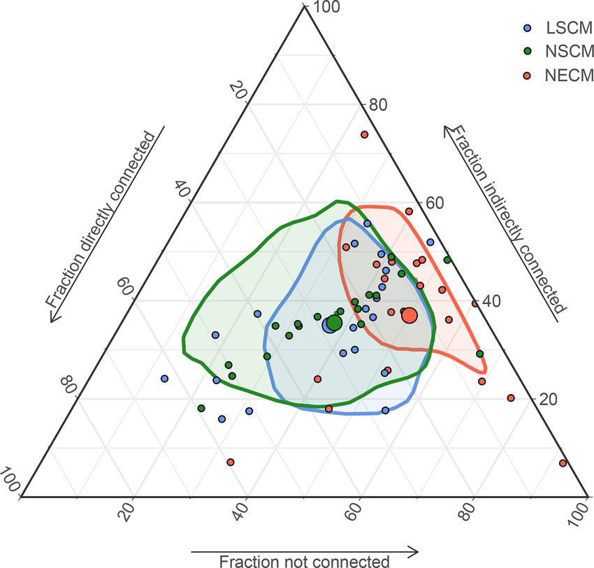
1730                   U. Schönenberger and C. Stamm: Hydraulic shortcuts connect arable land areas to surface waters

Table 1. Catchment properties of the 20 study areas. Fractions of agricultural area and of arable land were determined from BFS (2014), the
mean slope of agricultural areas was determined from BFS (2014) and Swisstopo (2018), and the mean annual precipitation was determined
from Kirchhofer and Sevruk (1992).

          ID   Location         Canton    Receiving             Area    Fraction of    Fraction of      Mean slope     Mean annual
                                          water                (km2 )   agricultural   arable land   of agricultural   precipitation
                                                                        area                            areas in the       (mm/yr)
                                                                                                     catchment (◦ )
          1    Böttstein        AG        Bruggbach              3.3    52 %           30 %                     8.5           1187
          2    Ueken            AG        Staffeleggbach         2.0    42 %           39 %                     7.6           1164
          3    Rüti b. R.       BE        Biberze                2.2    29 %           11 %                    11.2           1403
          4    Romont           FR        Glaney                 3.4    78 %           48 %                     4.0           1344
          5    Meyrin           GE        Nant d’Avril          10.0    49 %           31 %                     3.2           1133
          6    Boncourt         JU        Saivu                  5.9    44 %           23 %                     5.5           1093
          7    Courroux         JU        Canal de Bellevie      2.8    82 %           75 %                     2.9           1082
          8    Hochdorf         LU        Stägbach               2.4    84 %           59 %                     4.1           1213
          9    Müswangen        LU        Dorfbach               3.0    79 %           61 %                     4.0           1482
          10   Fleurier         NE        Buttes                 1.0    24 %           11 %                     9.6           1538
          11   Lommiswil        SO        Bellacher Weiher       3.8    50 %           40 %                     6.8           1388
          12   Illighausen      TG        Tobelbach              1.9    54 %           30 %                     1.8           1122
          13   Oberneunforn     TG        Brüelbach              3.3    69 %           52 %                     4.2            968
          14   Clarmont         VD        Morges                 2.4    75 %           70 %                     5.3           1163
          15   Molondin         VD        Flonzel                4.2    74 %           65 %                     5.9           1064
          16   Suchy            VD        Ruiss. des Combes      3.3    72 %           63 %                     5.6           1026
          17   Vufflens         VD        Venoge                 2.8    39 %           30 %                     5.7           1006
          18   Buchs            ZH        Furtbach               3.9    57 %           48 %                     4.9           1182
          19   Nürensdorf       ZH        Altbach                2.3    59 %           44 %                     3.6           1225
          20   Truttikon        ZH        Niederwisenbach        5.1    66 %           49 %                     4.6            960
                                          Mean                   3.5    59 %           44 %                     4.9           1159

     a visible light camera (Sony DSC-WX220; RGB). The                  2.2.3    Assigning shortcuts to landscape elements
     study areas were fully covered by the UAV imagery,
     with the exception of larger settlement areas, forests,            In order to better understand where hydraulic shortcuts oc-
     lakes, and no-fly zones for drones (e.g. airports). The            cur the most, we assigned them to different landscape ele-
     UAV images were processed to one georeferenced aerial              ments. Using the topographic landscape model of Switzer-
     image per study area using the software Pix4Dmapper                land, swissTLM3D (Swisstopo, 2010), we defined five land-
     4.2. In the no-fly zones of the study areas in Meyrin              scape elements, namely paved roads, unpaved roads, fields,
     (Geneva), Buchs (Zürich), and Nürensdorf (Zürich), we              settlements, and other areas (e.g. railways, other traffic ar-
     used aerial images provided by the cantons of Geneva               eas, forests, water bodies, wetlands, and single buildings).
     (Etat de Genève, 2016) and Zürich (Kanton Zürich,                  For all landscape elements except roads and railways, short-
     2015). Ground resolutions were 5 and 10 cm respec-                 cuts were assigned to their landscape elements by a simple
     tively. Using ArcGIS 10.7, we gridded the aerial im-               intersection. However, shortcuts belonging to road or rail-
     ages, scanned by eye through each of the grid cells,               way drainage systems are, in many cases, not placed directly
     and marked all potential shortcut structures manually.             on the road or railway but on the adjacent agricultural land
     If observable from the aerial image, the same properties           or settlement. Therefore, shortcuts were assigned to the land-
     as for the field survey were specified for each potential          scape elements of road or railway if they were within a 5 m
     shortcut structure.                                                buffer.
                                                                           In addition, we correlated the density of shortcuts per
     We combined the three data sets originating from the               study area to different study area properties. We selected
     three methods to a single data set. If a potential shortcut        properties that we expected to have explanatory power, i.e.
     structure was only found by one of the mapping meth-               density (length per area) of paved roads, density of unpaved
     ods, its location and type were used for the combined              roads, density of surface rivers, density of subsurface rivers,
     data set. If it was found by more than one of the map-             mean annual precipitation, and mean slope on agricultural
     ping methods, we used the location and type of the map-            areas.
     ping method that we expected to be the most accurate.
     For the location information and the type specification,
     we used UAV imagery, before field survey, and maps.

Hydrol. Earth Syst. Sci., 25, 1727–1746, 2021                                              https://doi.org/10.5194/hess-25-1727-2021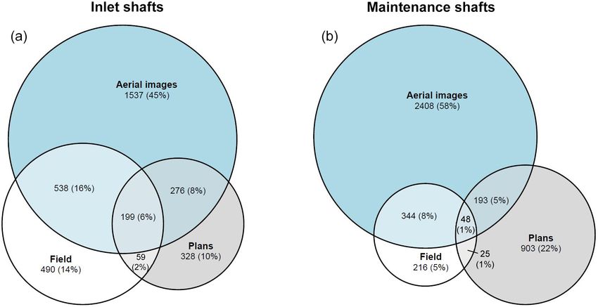
U. Schönenberger and C. Stamm: Hydraulic shortcuts connect arable land areas to surface waters                                  1731

2.2.4    Drainage of shortcuts                                         Recipient areas. Surface runoff generated on a source area
                                                                    and routed through the landscape can end up in three dif-
A potential shortcut only turns into a real one if it is drained    ferent types of landscape elements, referred to as recipient
to surface waters by pipes or other connecting structures such      areas, namely surface waters, infiltration areas (i.e. forests,
as ditches. Therefore, using the plans provided by the mu-          hedges, and internal sinks), and shortcuts. The extent of
nicipalities, we investigated where potential shortcuts drain       surface waters (rivers that have their course above the sur-
to. They were allocated to one of the following categories          face, lakes, and wetlands), was defined by the swissTLM3D
of recipient areas, namely surface waters, wastewater treat-        model, as was the extent of forests and hedges. Since forests
ment plants and/or combined sewer overflows, infiltration ar-       and hedges are known to infiltrate surface runoff (Sweeney
eas (e.g. forests, infiltration ponds, fields, and grassland), or   and Newbold, 2014; Schultz et al., 2004; Bunzel et al., 2014;
unknown.                                                            Dosskey et al., 2005), we assumed that forests with a cer-
                                                                    tain width (parameter–infiltration width) act as an infiltration
2.3     Surface runoff connectivity model                           area. Hedges were assumed to either act as infiltration areas
                                                                    or to have no effect on surface runoff. Accordingly, the pa-
To assess how hydraulic shortcuts contribute to surface
                                                                    rameter hedge infiltration was varied between yes (hedges act
runoff connectivity, we created a surface runoff connectivity
                                                                    as infiltration areas) and no (hedges do not act as an infiltra-
model.
                                                                    tion areas).
   The model is based on the concept of critical source ar-
                                                                       Internal sinks in the landscape were defined using the
eas (CSAs; see introduction). It mainly focuses on the first
                                                                    2×2 m digital elevation model (DEM; Swisstopo, 2018). All
two elements of the CSA concept (i.e. pesticide application
                                                                    sinks larger than two raster cells and deeper than a certain
and connectivity to surface waters). In contrast, the ques-
                                                                    depth (parameter–sink depth) were defined as internal sinks.
tion of whether an area is hydrologically active is only ad-
                                                                    All other sinks were filled completely.
dressed partially because much relevant information, such as
                                                                       Shortcuts were defined in two different ways (parameter –
soil properties, is not available at the national scale.
                                                                    shortcut definition). In definition A, all inlet shafts, ditches,
   The model (see Fig. 2) distinguishes source areas on which
                                                                    and channel drains were considered as potential shortcuts.
surface runoff is produced, and recipient areas on which sur-
                                                                    In definition B, maintenance shafts lying in internal sinks
face runoff ends up. A connectivity model connects those ar-
                                                                    were additionally considered as potential shortcuts. Poten-
eas by routing surface runoff through the landscape. These
                                                                    tial shortcuts were defined to act as real shortcuts if they are
model parts are conceptually described in more detail in
                                                                    known to discharge to surface waters or wastewater treat-
Sect. 2.3.1. In Sect. 2.3.2, we describe how we parameterized
                                                                    ment plants. From the drainage plans of the municipalities,
the model, and how we assessed the uncertainty of model
                                                                    we know that most of the inlet shafts discharge into either
output given the parameter uncertainty. In Sect. 2.3.3, we ex-
                                                                    a surface water body or a wastewater treatment plant. There-
plain the testing for systematic differences in the hydrologi-
                                                                    fore, also potential shortcuts with unknown drainage location
cal activity between areas with direct or indirect connectivity.
                                                                    were assumed to act as real shortcuts. Potential shortcuts dis-
2.3.1    Model structure                                            charging into forests or infiltration structures were assumed
                                                                    not to act as shortcuts and were not used in the model. Short-
Source areas. All crop areas on which pesticides are applied        cut recipient areas were defined as the raster cells of the dig-
should, in theory, be considered as source areas. However,          ital elevation model on which the shortcut is located and all
a highly resolved spatial data set of land in a crop rota-          the cells directly surrounding it (see Fig. S14 in the Supple-
tion for our study areas is lacking. Therefore, we considered       ment).
the total extent of agricultural areas (i.e. arable land, mead-        Connectivity model. For modelling connectivity, we used
ows and/or pastures, vineyards, orchards, and gardening) as         the TauDEM model (Tarboton, 1997), which is based on a
source areas, since those areas could be derived in high res-       D-infinity flow direction approach. As an input, we used a
olution. The extent of agricultural areas was defined by sub-       2×2 m digital elevation model (Swisstopo, 2018). This DEM
tracting all non-agricultural areas from the extent of the study    was modified as follows. We assumed that only those inter-
area. For this, we used non-agricultural areas (forests, water      nal sinks that were defined as sink recipient areas (see above)
bodies, urban areas, traffic areas, and other non-agricultural      effectively act as sinks. Therefore, first, all sinks were filled,
areas) as defined by the national topographical landscape           and sink recipient areas were carved 10 m into the DEM. Sec-
model swissTLM3D (Swisstopo, 2010). According to the                ond, all other recipient areas (shortcuts, forests, hedges, and
Swiss proof of ecological performance (PEP), pesticide us-          surface waters) were carved between 10 and 50 m into the
age within a distance of 6 m from a river and within 3 m from       DEM. Carving the recipient areas into the DEM ensured that
hedges and forests is prohibited. The extent of agricultural        surface runoff reaching a recipient area was not routed fur-
areas was reduced accordingly, except along forests (param-         ther on to another recipient area. Third, to account for the
eters – river spray buffer and hedge spray buffer).                 effect of roads accumulating surface runoff (Heathwaite et

https://doi.org/10.5194/hess-25-1727-2021                                        Hydrol. Earth Syst. Sci., 25, 1727–1746, 2021
1732                   U. Schönenberger and C. Stamm: Hydraulic shortcuts connect arable land areas to surface waters

Figure 2. Structure of the surface runoff connectivity model. WWTPs – wastewater treatment plants; CSO – combined sewer overflow.

al., 2005), roads were carved into the DEM by a given depth          we selected the values that we assumed to be the most prob-
defined by the parameter road carving depth.                         able in reality. For the local sensitivity analysis, each of the
   The modified DEM, the source areas, and the recipient ar-         model parameters was varied individually within the same
eas were used as an input into the TauDEM tool of D-infinity         boundaries as for the Monte Carlo analysis.
upslope dependence. In this way, each raster cell belonging
to a source area was assigned with the probability of being          2.3.3   Hydrological activity
drained into one of the three types of recipient areas.
   The connectivity of a source area may depend on the flow          As mentioned earlier, a critical source area has to be hydro-
distance to surface waters. For longer flow distances, water         logically active, i.e. surface runoff has to be generated on that
has a higher probability of infiltrating before it reaches a sur-    area. Runoff generation depends on many variables (e.g. crop
face water. Therefore, for each source area raster cell, we cal-     types, soil types, soil moisture, and rain intensity) for which
culated the flow distance to its recipient area using the tool       no data are available in most of our study areas and which
D-infinity distance down.                                            are strongly variable over time. Since we are interested in the
                                                                     general relevance of shortcuts, we focused on the question
2.3.2   Model parametrization and sensitivity analyses               of whether there is a systematic difference in the hydrologi-
                                                                     cal activity between areas directly or indirectly connected to
The model parameters mentioned in the section above vary in          streams.
space and time. Since this variability could not be addressed           For soil moisture, we tested for such differences by cal-
with the selection of a single parameter value, we performed         culating the distribution of the topographic wetness index
a Monte Carlo simulation with 100 realizations. The proba-           (TWI; Beven and Kirkby, 1979) for the source areas of the
bility distributions of the parameters are provided in Table 2.      benchmark model. We calculated the TWI as follows, using
The bounds or categories of these distributions were based           the tool in the TauDEM model:
on our prior knowledge about the hydrological processes in-                    ln (a)
volved, about structural aspects (e.g. depths of sinks), and         TWI =            .                                             (1)
                                                                              tan (β)
on our experience from field mapping. The parameters river
spray buffer and hedge spray buffer were assumed constant            The local upslope area a and the local slope β were calcu-
according to the guidelines of the Swiss proof of ecological         lated using the D-infinity flow direction algorithm that was
performance (PEP).                                                   already used for the surface runoff connectivity model. As
   To assess the influence of single parameters on our mod-          an input, we used the source areas and the modified DEM as
elling results, we performed a local sensitivity analysis            specified for the surface runoff connectivity model.
against a benchmark model (one realization of the model                 The formation of surface runoff on agricultural areas is
with a specific parameter set; see Table 2). When selecting          also influenced by their slope. Therefore, we calculated the
the benchmark model parameter set, we kept the changes in            distribution of slopes for source areas draining to different
the digital elevation model small (i.e. road carving depth is        destinations. For this, we used the slopes from the Swiss dig-
0 cm; sink depth is 10 cm). For the other model parameters,          ital elevation model (Swisstopo, 2018).

Hydrol. Earth Syst. Sci., 25, 1727–1746, 2021                                             https://doi.org/10.5194/hess-25-1727-2021
U. Schönenberger and C. Stamm: Hydraulic shortcuts connect arable land areas to surface waters 1733
Table 2. Summary of parameter distributions used for the Monte Carlo analysis and parameter values used as a benchmark for the sensitivity
analysis. PEP – Swiss proof of ecological performance.
Parameter Handling of parameter uncertainty Distribution Bounds/categories Benchmark model
Sink depth Monte Carlo and sensitivity analysis Uniform distribution 5 cm ≤ x ≤ 100 cm 10 cm
Infiltration width Monte Carlo and sensitivity analysis Uniform distribution 6 m ≤ x ≤ 100 m 20 m
Road carving depth Monte Carlo and sensitivity analysis Uniform distribution 0 cm ≤ x ≤ 100 cm 0 cm
Shortcut definition Monte Carlo and sensitivity analysis Bernoulli distribution (Definition A; definition B) Definition A
Hedge infiltration Monte Carlo and sensitivity analysis Bernoulli distribution (Yes; no) Yes
River spray buffer Assumed as certain; based on PEP guidelines Constant 6m 6m
Hedge spray buffer Assumed as certain; based on PEP guidelines Constant 3m 3m
For other variables (e.g. crop type and rain intensity), there in Fig. 3. Mathematical details are provided in the Supple-
is no indication of such systematic differences. Therefore, we ment (Sect. S1.5).
assumed that they do not differ systematically between areas As a result, we obtained a national surface runoff con-
draining to different recipient areas. nectivity model (NSCM). The NSCM provides an estimate
for the fractions of agricultural areas directly, indirectly, and
not connected to surface waters (fNSCM,dir , fNSCM,indir , and
2.4 Extrapolation to the national level
fNSCM,nc ) for the catchments of the national catchment data
set. Since mountainous regions of higher altitudes are ex-
2.4.1 Extrapolation of the local connectivity model cluded in the NECM, those areas are also excluded in the
NSCM.
In a last step, we developed a model to extrapolate the results
2.4.2 Connectivity of crop areas
from our study areas (local surface runoff connectivity model
– LSCM) to the national scale. This extrapolation was then During the time of this study, high-resolution data sets of
used to evaluate how the results of this study compare to a Swiss crop areas were not available in Switzerland. There-
pre-existing connectivity model (national erosion connectiv- fore, we considered the total extent of agricultural areas for
ity model – NECM; Alder et al., 2015). building the local surface runoff connectivity model and ex-
Selection of explanatory variables. We calculated a list of trapolation to the national scale. This includes areas with rare
catchment statistics based on nationally available geo-data pesticide application, such as meadows and pastures.
sets that could serve as explanatory variables. As catchment The Swiss land use statistics data set (BFS, 2014) is a
boundaries, the polygons from the national catchment data raster data set with a resolution of 100 m, dividing agricul-
set (BAFU, 2012) were used. Details on the data sets used tural areas into different categories (e.g. arable land, vine-
for calculating those catchment statistics can be found in Ta- yards, and meadows and/or pastures). On the national scale,
ble S1. the use of such a lower-resolution data set is more reason-
We created a linear regression between each of those able. Hence, we used this data set to calculate fractions of
catchment statistics to the median fractions of agricultural ar- connected crop areas.
eas directly, indirectly, and not connected to surface waters, The fractions of directly, indirectly, and not connected
as reported by the LSCM (fLSCM,dir , fLSCM,indir , fLSCM,nc ). crop areas per total agricultural area per catchment c
The strongest correlations were found for the fractions of (fNSCM,crop,c ) were calculated as follows:
agricultural areas directly, indirectly, and not connected
to surface waters, as reported by the NECM (fNECM,dir , fNSCM,crop,c = fNSCM,c · rcrop,c , (2)
fNECM,indir , and fNECM,nc ; see Table S8). Therefore, we used
them as explanatory variables to build an extrapolation model with rcrop being the ratio of crop area to total agricultural area
of our local results to the national scale. in a catchment, as follows:
The model predictions for each catchment have to fulfil
specific boundary conditions. First, the sum of areal fractions Acrop,c
rcrop,c = (3)
of the three Ptypes of recipient areas k per catchment c has to Acrop,c + Amead,c
equal one ( K k=1 fk,c = 1), and second, area fractions can- Acrop,c = Aarab,c + Avin,c + Aorch,c + Agard,c , (4)
not be negative (fk,c ≥ 0). To ensure these conditions, we
performed the model fit after a unit simplex data transforma- where, in catchment c, Acrop,c is the crop area, Amead,c is
tion. To address the uncertainty introduced by the selection the meadow and pasture area, Aarab,c is the arable land area,
of our study catchments, we additionally bootstrapped the Avin,c is the vineyard area, Aorch,c is the orchard area, and
model 100 times. The resulting modelling approach is shown Agard,c is the gardening area.
https://doi.org/10.5194/hess-25-1727-2021 Hydrol. Earth Syst. Sci., 25, 1727–1746, 20211734 U. Schönenberger and C. Stamm: Hydraulic shortcuts connect arable land areas to surface waters
Figure 3. Extrapolation of the local surface runoff connectivity model (LSCM) to the national scale (NSCM) using a unit simplex transfor-
mation approach. Equations (2)–(4) are shown in Sect. 2.4.2. Equations (S2)–(S5) are provided in the supplement (Sect. S1.5).
3 Results therefore, less often on paved or unpaved roads. The fractions
of inlet and maintenance shafts belonging to a certain land-
3.1 Occurrence of hydraulic shortcuts scape element for each study area can be found in Figs. S17
and S18.
In the following section, we first show the results of the field We correlated the densities of inlet and maintenance shafts
mapping campaign for shafts (inlet and maintenance shafts), per study area with possible explanatory variables. Only the
followed by the results for channel drains and ditches. Af- density of paved roads was significantly correlated to the
terwards, we present results on the accuracy of our mapping density of inlet shafts (R 2 = 0.33; p = 0.008) and mainte-
methods. nance shafts (R 2 = 0.37; p = 0.005; see Tables S6 and S7).
3.1.1 Shafts 3.1.2 Channel drains and ditches
In total, we found 8213 shafts, corresponding to an average In addition to shafts, we also mapped channel drains and
shaft density of 2.0 ha−1 (min – 0.51 ha−1 ; max – 4.4 ha−1 ; ditches. With the exception of the study areas Meyrin
Table 3). A total of 42 % of the shafts mapped were in- (4.2 m ha−1 ) and Buchs (4.0 m ha−1 ), these structures were
let shafts. A plot showing the density of shafts mapped per rarely found (< 1.2 m ha−1 ; see Fig. S16). In Meyrin and
catchment and shaft type can be found in Fig. S15. Buchs, most channel drains and ditches (98 % of the total
For roughly half of the inlet and maintenance shafts, we length) drain to surface waters, and only few of them to infil-
were able to identify a drainage location. Both shaft types tration areas (2 %).
discharge in almost all cases into surface waters, either di-
rectly (87 % of inlet shafts; 63 % of maintenance shafts) or 3.1.3 Mapping accuracy
via wastewater treatment plants or combined sewer over-
flows (12 % of inlet shafts; 37 % of maintenance shafts). The results above were generated using three different map-
Only 1.4 % of the inlet shafts and no maintenance shaft at ping methods (field survey, aerial images, and drainage
all, were found to drain to an infiltration area such as forests plans). These methods differ in their ability to identify and
or fields. classify a potential shortcut structure correctly and in the
Most of the inlet shafts mapped (90 %) are located on study area they cover. We determined the accuracy of the
paved or unpaved roads (see Table 4). Only very few in- mapping methods for aerial images and drainage plans using
let shafts (2.8 %) are found directly on fields. In contrast, the field survey method as a ground truth (see Table 5) for
maintenance shafts are found much more often on fields and, those parts of the study areas where all three methods were
Hydrol. Earth Syst. Sci., 25, 1727–1746, 2021 https://doi.org/10.5194/hess-25-1727-2021U. Schönenberger and C. Stamm: Hydraulic shortcuts connect arable land areas to surface waters 1735
Table 3. Number of shafts found in agricultural areas of the study areas per shortcut category and drainage location. WWTP – wastewater
treatment plant; CSO – combined sewer overflow.
Inlet shafts Maintenance shafts Other shafts Unknown type
Drainage location Count Fraction Count Fraction Count Fraction Count Fraction
Surface waters 1568 46 % 1205 29 % 0 0% 0 0%
WWTP/CSO 218 6% 705 17 % 0 0% 0 0%
Infiltration areas 26 1% 0 0% 0 0% 0 0%
Unknown 1615 47 % 2227 54 % 31 100 % 618 100 %
Total 3427 100 % 4137 100 % 31 100 % 618 100 %
Table 4. Percentage of shafts found in a certain type of landscape element. The category of other areas integrates several types of landscape
elements, including railways, other traffic areas, forests, water bodies, wetlands, and single buildings.
Paved Unpaved Settle- Fields Other
roads roads ments areas
Inlet shafts 79 % 10 % 5.5 % 2.8 % 2.2 %
Maintenance shafts 52 % 7.2 % 16 % 21 % 4.5 %
applied. Since channel drains and ditches were rare, this as- Molondin. These simulations correspond to the 5 %, 50 %,
sessment was only performed for shafts. and 95 % quantile of the median fraction of indirectly con-
The recall (i.e. the probability that a potential shortcut is nected per total connected agricultural area over all study
found by a mapping method) was limited for the aerial im- catchments. The classification of certain catchment parts is
ages method (53 % for inlet shafts; 62 % for maintenance changing, depending on the model parameterization (e.g. let-
shafts) and even lower for the drainage plans method (32 % ters A to C). However, for other parts, the results are con-
for inlet shafts; 21 % for maintenance shafts). However, iden- sistent across the different MC simulations (e.g. letters D to
tified shortcuts were, in most of the cases, classified correctly F). Overall, the results show that not only agricultural areas
(accuracy – 93 % to 94 % for aerial images; 88 % to 89 % for close to surface waters (e.g. letter D) are connected to sur-
drainage plans). face waters. Hydraulic shortcuts also create surface runoff
For the entire study area, Fig. 4 shows the number of po- connectivity for areas far away from surface waters (e.g. let-
tential shortcuts identified by the three mapping methods. ter E).
Despite a low recall, aerial images identified the largest num- In order to assess the importance of hydraulic shortcuts,
ber of potential shortcuts. This is due to the large spatial cov- we calculated the fraction of the indirectly connected area
erage by the aerial images method. Since the overlap between to the total connected area. Across all Monte Carlo simula-
the three methods is small (only 32 % of the inlet shafts and tions, the median of this fraction over all study catchments
15 % of the maintenance shafts were found by more than one ranges between 43 % and 74 % (mean – 57 %; median –
method), each of the methods was important for determining 58 %; Fig. 6). Despite considerable uncertainty, the results
the total number of potential shortcuts in the study areas. Be- demonstrate that a large fraction of the surface runoff con-
cause the aerial images and drainage plans have a low recall nectivity to surface waters is established by hydraulic short-
but cover large parts of the study areas that were not assessed cuts.
by the field survey, the numbers reported above are a lower For different flow distances, the fraction of indirectly con-
boundary estimate. nected area to the total connected area underlies only mi-
nor variations (see Fig. S24). However, this fraction varies
3.2 Surface runoff connectivity strongly between the study areas, with median fractions rang-
ing from 21 % in Müswangen to 97 % in Boncourt. Although
3.2.1 Study areas the occurrence of hydraulic shortcuts is a prerequisite for in-
direct connectivity, high shaft densities are not necessarily
From the Monte Carlo analysis of the surface runoff con- leading to high fractions of indirect connectivity in a catch-
nectivity model, we obtained an estimate for the fractions of ment. The densities of inlet and maintenance shafts show
agricultural areas that are connected directly, indirectly, or only a weak positive correlation to the catchment medians
not at all to surface waters. To illustrate the variability result- of the fraction of indirectly connected areas (inlet shafts –
ing from these Monte Carlo (MC) runs, Fig. 5 shows the out- R 2 = 0.11 and p = 0.15; maintenance shafts – R 2 = 0.08 and
put of three MC simulations (MC28, MC41, and MC40) for
https://doi.org/10.5194/hess-25-1727-2021 Hydrol. Earth Syst. Sci., 25, 1727–1746, 20211736 U. Schönenberger and C. Stamm: Hydraulic shortcuts connect arable land areas to surface waters
Table 5. Recall and classification accuracies of the mapping methods of aerial images and drainage plans. The recall corresponds to the
probability that a potential shortcut is found by the mapping method. Percentages indicate the recall of each individual mapping method. In
parentheses, the recall of the combination of both methods is given. The accuracy corresponds to the sum of true positive fraction and true
negative fraction.
Mapping method Shaft type Identification Classification
Recall True False True False Accuracy
positives positives negatives negatives
Aerial images Inlet shafts 53 % (60 %) 61 % 1.3 % 33 % 4.9 % 94 %
Maintenance shafts 62 % (69 %) 32 % 5.3 % 61 % 1.3 % 93 %
Drainage plans Inlet shafts 32 % (60 %) 67 % 4.5 % 22 % 6.6 % 89 %
Maintenance shafts 21 % (69 %) 20 % 7.1 % 68 % 5.3 % 88 %
Figure 4. Number of inlet (a) and maintenance shafts (b) identified by the different mapping methods.
p = 0.23; see Table S8). By contrast, the two study areas with a large influence on the estimated fractions of direct and in-
high channel drain and ditch densities (Meyrin and Buchs) direct connectivity.
show high fractions of indirect connectivity. Similarly, the So far, we only reported on the fraction of indirectly con-
density of surface waters is strongly negatively correlated to nected per total connected area. In Table 6, we additionally
the fraction of indirect connectivity (R 2 = 0.51; p < 0.001). report the fractions of total agricultural area connected di-
This suggests that line elements like channel drains, ditches, rectly, indirectly, and not at all to surface waters. On aver-
and surface waters usually have an influence on connectiv- age, we estimate between 5.5 % and 38 % (mean – 28 %) of
ity if they occur in a catchment. In contrast, the influence the agricultural area to be connected directly, 13 % to 51 %
of point elements seems to depend a lot on the surrounding (mean – 35 %) to be connected indirectly, and 12 % to 77 %
landscape structure. (mean – 37 %) not to be connected to surface waters. How-
As a further consequence of the structural differences be- ever, the variation between the catchments is much larger
tween the study areas, not all of them reacted the same way than the variation of the Monte Carlo analysis.
to changes in model parameters of the Monte Carlo anal-
ysis. For example, the fraction of indirectly to total con- 3.2.2 Sensitivity analysis
nected areas in the study area Boncourt was quite insensitive
to changes in model parameters. Since Boncourt has a very To analyse which model parameters have the largest influ-
low water body density, only small areas are connected di- ence on our model results, we tested the local model param-
rectly, which is independent of the model parameterization. eter sensitivity on our benchmark model. The fraction of in-
The study area Illighausen, on the other hand, reacted very directly to total connected area has the most sensitive reac-
sensitively (range of results – 68 %). Since Illighausen is a tion to changes in the road carving depth parameter. The dif-
very flat catchment, changes in the sink depth parameter had ference between the minimal and maximal fraction reported
Hydrol. Earth Syst. Sci., 25, 1727–1746, 2021 https://doi.org/10.5194/hess-25-1727-2021U. Schönenberger and C. Stamm: Hydraulic shortcuts connect arable land areas to surface waters 1737
Figure 5. Results of three example Monte Carlo (MC) simulations for a part of one study area (Molondin). The colour ramps show the
probability of agricultural areas to be directly connected (blue), indirectly connected (red), and not connected (green). The simulations
represent, approximately, the 5 % (MC28), 50 % (MC41), and 95 % (MC40) quantiles with respect to the resulting median fractions of
indirectly connected per total connected area over all study catchments. The parameters of the example MC simulations are shown at the
bottom right. Source of background map: Swisstopo (2010).
Figure 6. (a) Fractions of indirectly connected areas per total connected areas as calculated by the Monte Carlo analysis for each study
area. White dots indicate the means of the distributions. The red dots indicate the results of the example Monte Carlo simulations (MC28,
MC41, and MC 40) shown in Fig. 5. (b) Distribution of medians of fractions of indirectly connected areas per total connected areas per study
catchment and per Monte Carlo simulation.
was 17 %. Results were also sensitive to the parameters short- 3.2.3 Hydrological activity
cut definition (14 %) and sink depth (13 %). Infiltration width
(4.3 %) and hedge infiltration (2.5 %) had only a minor influ- Systematic differences in hydrological activity between di-
ence on the fraction reported (see Figs. S22 and S23). rectly and indirectly connected areas would have a major in-
fluence on the interpretation of our connectivity analysis. We,
therefore, tested for such differences by calculating the dis-
tributions of slope and topographic wetness index on these
areas.
https://doi.org/10.5194/hess-25-1727-2021 Hydrol. Earth Syst. Sci., 25, 1727–1746, 20211738 U. Schönenberger and C. Stamm: Hydraulic shortcuts connect arable land areas to surface waters
Table 6. Fractions of directly, indirectly, and not connected agricultural areas in our study catchments. The first row represents the mean
fraction over all catchments and Monte Carlo simulations. The second row represents the median of the median over all catchments per MC
simulation. The third row represents the median of the median over all MC analyses per catchment. In parentheses, the minimum and the
maximum median are given.
Statistic Fraction of directly Fraction of indirectly Fraction of not Fraction of indirectly
connected agricultural connected agricultural connected agricultural per total connected area
area fdir area findir area fnc ffracindir
Mean 28 % 35 % 37 % 57 %
Median per MC simulation 25 % (5.5 %; 38 %) 38 % (13 %; 51 %) 32 % (12 %; 77 %) 58 % (43 %; 74 %)
Median per catchment 26 % (1.8 %; 70 %) 37 % (12 %; 60 %) 35 % (3.9 %; 53 %) 57 % (21 %; 97 %)
The distributions of both slope and topographic wetness
index were very similar for directly, indirectly, and not con-
nected areas (see Figs. S25 and S26). Only the slope of not
connected areas was found to be slightly smaller than the
slope of connected areas. Hence, we could not identify any
systematic differences in the factors affecting hydrological
activity between directly and indirectly connected areas.
Consequently, given the current knowledge, the propor-
tions of direct and indirect surface runoff entering surface
waters are expected to be equal to the proportions of directly
and indirectly connected agricultural areas. Analogously, if
other boundary conditions of pesticide transport remain un-
changed, directly and indirectly transported pesticide loads
are expected to be proportional to directly and indirectly con-
nected crop areas.
3.2.4 Extrapolation to the national level
We created a model for extrapolating the results of our study
areas to the national level, using area fractions of the national
erosion connectivity model (NECM; Alder et al., 2015) ag- Figure 7. Fractions (%) of directly connected (fdir ), indirectly con-
gregated to the catchment scale as explanatory variables. The nected (findir ), and not connected areas (fnc ) per total agricultural
area fractions of the NECM were transformed such that they area for the local surface runoff connectivity model (LSCM; blue),
national erosion connectivity model (NECM; red), and national sur-
fit the area fractions of the local surface runoff connectivity
face runoff connectivity model (NSCM; green) in the 20 study ar-
model (LSCM) resulting from the Monte Carlo analysis in
eas. Small blue circles represent the catchment medians of all Monte
our study areas. The resulting data set is called the national Carlo simulations of the LSCM, small red circles represent the data
surface runoff connectivity model (NSCM). The NSCM pro- reported by the NECM, and small green circles represent the catch-
vides a separate model for each of the 100 Monte Carlo runs ment medians of the NSCM. Large circles represent the means of
of the LSCM. It is aggregated to the catchment scale and cov- the LSCM (blue), NECM (red), and NSCM data (green). Shaded ar-
ers all catchments of the valley zones, hill zones, and lower eas represent normal kernel density estimates of the LSCM, NECM,
elevation mountain zones. The differences between the fitted and NSCM data.
NSCM and the LSCM were strongly reduced compared to
the original NECM (see Fig. 7). The root mean square error
(RMSE), on average, reduced from 17 % to 9.5 % for directly average, 26 % of crop areas (13 % of total agricultural area)
connected fractions, from 12 % to 7.6 % for indirectly con- are connected directly, 34 % (17 % of total agricultural area)
nected fractions, and from 18 % to 7.6 % for not connected indirectly, and 40 % (20 % of total agricultural area) not at
fractions. all (see Fig. S27 for details; for MC simulation quantiles, see
By combining the NSCM with land use data, we came Table S9; for spatial distribution, see Figs. S30 to S36). From
up with an estimate of connected crop areas on the national the total connected crop area, 54 % (between 47 % and 60 %)
scale. Half of the Swiss agricultural areas in the model region are connected indirectly.
are crop areas (i.e. arable land, vineyards, orchards, and hor- These results are similar to those obtained for the 20 study
ticulture) and, therefore, potential pesticide source areas. On areas. Mean fractions of directly and indirectly connected
Hydrol. Earth Syst. Sci., 25, 1727–1746, 2021 https://doi.org/10.5194/hess-25-1727-2021U. Schönenberger and C. Stamm: Hydraulic shortcuts connect arable land areas to surface waters 1739
agricultural areas are a bit smaller in the national scale es- only other study in Switzerland reporting numbers on storm
timation than for the 20 study areas (−2.0 % and −1.9 %), drainage inlet shafts (Prasuhn and Grünig, 2001).
while the fraction of not connected agricultural area is a bit The vast majority of mapped storm drainage inlet shafts
larger (+3 %). The fraction of indirectly connected crop area were found to discharge to surface waters directly or via
per total connected crop area is slightly smaller (−2.6 %). wastewater treatment plants (WWTPs). Thus, the occurrence
To assess if the national erosion connectivity model of an inlet shaft is, in most cases, directly related to a risk
(NECM) is different from the national surface runoff con- for pesticide transport to surface waters. The following three
nectivity model (NSCM), we determined the 5 % and 95 % processes generate this risk. First, pesticide-loaded surface
quantiles of the NSCM predictions (see Table S9). If a frac- runoff produced on crop areas can enter the inlet shaft. Sec-
tion of the NECM is outside of this range, we considered ond, spray drift deposited on roads can be washed off and en-
this as a significantly different model prediction that is not ter the inlet shaft. Third, inlet shafts can be oversprayed dur-
expected given our field data. ing pesticide application, which is mainly considered proba-
Compared to the NSCM, the NECM, on average, pre- ble for inlet shafts located in the fields.
dicts lower fractions of directly connected crop areas fcrop,dir Although maintenance shafts were also found to discharge
(−6.4 %), which is below the 5 % quantile of the NSCM re- to surface waters directly or via WWTPs, their occurrence
sults. For indirectly connected areas fcrop,indir (−0.9 %) and does not directly translate into a risk for pesticide transport
not connected crop areas fcrop,nc (+7.2 %), the data reported to surface waters. In contrast to storm drainage inlet shafts,
by the NECM are within the 5 % and 95 % quantile of the maintenance shafts are not designed to collect surface runoff.
NSCM results. However, the fraction of indirectly connected Their lids are usually closed or only have a small opening,
crop area per total connected crop area ffracindir reported significantly decreasing the risk of either surface runoff en-
by the NECM lies beyond the 95 % quantile of the NSCM tering the maintenance hole or of overspraying. In addition,
(+11 %). In summary, fcrop,dir and ffracindir reported by the lids of maintenance shafts in fields are often elevated com-
NECM are significantly different from what would be ex- pared to the soil surface. Maintenance shafts on roads are
pected from the NSCM. For fcrop,indir and fcrop,nc , the re- (in contrast to inlet shafts) usually positioned so that concen-
ported fractions are in a similar range for both models. The trated surface runoff bypasses them. However, as also shown
results of the bootstrap (Fig. S28) show that the differences by Doppler et al. (2012), maintenance shafts can collect sur-
between the two models are significantly larger than the un- face runoff from fields if they are located in a sink or a thal-
certainty introduced by the selection of the study catchments. weg and water is ponding above them during rain events.
The average difference in predicted connectivity frac- During our field mapping campaign, we additionally found
tions of agricultural areas between the two models several damaged maintenance shafts that could easily act as
(1f = ((fNSCM,dir −fNECM,dir )+(fNSCM,indir −fNECM,indir ) a shortcut.
+(fNSCM,nc − fNECM,nc ))/3) is strongly variable in space. Channel drains and ditches discharging into surface wa-
Large differences are mainly found in large valleys (e.g. ters were rare in most study areas, with two exceptions. In
the Aare, Alpenrhein, and Rhône valleys and the valleys of Meyrin, the large length of these structures can be explained
Ticino) and in the region of Lake Constance (see Fig. S40). by the existence of a large vineyard. Additionally, the shaft
However, when looking at the difference in average pre- density in this vineyard was higher than on the surround-
dicted connectivity fractions of crop areas (1fcrop = ing arable land. This indicates that vineyards could gener-
((fNSCM,crop,dir − fNECM,crop,dir ) + (fNSCM,crop,indir − ally have higher shortcut densities than arable land. In Buchs,
fNECM,crop,indir ) + (fNSCM,crop,nc − fNECM,crop,nc ))/3), large around 60 % of the channel drain and ditch length consists
differences are almost exclusively found in a band of of ditches that cannot be clearly distinguished from small
catchments with high crop densities spreading through the streams. They are not appearing in the national topographic
Swiss midlands (see Fig. 8). landscape model (Swisstopo, 2010) that was used for the def-
inition of rivers and streams and did not appear to be streams
during field mapping or when analysing aerial images.
4 Discussion The number of mapped shortcuts represents a lower
boundary estimate of the shortcuts present (see Sect. 3.1.3)
4.1 Occurrence of hydraulic shortcuts and, therefore, leads to an underestimation of indirect con-
nectivity. Probabilities for missing shortcuts during our map-
Our study shows that storm drainage inlet and maintenance ping campaign depend on their location. While aerial im-
shafts are common structures found in Swiss agricultural ar- ages were at almost full coverage of the study areas, field
eas. While in neighbouring countries roads are often drained mapping was performed mainly along roads. Drainage plans
by ditches, Swiss roads are usually drained by storm drainage were available more often along roads than on fields. There-
inlet shafts (Alder et al., 2015). It is, therefore, not surpris- fore, we expect that the detection probability of shortcuts is
ing that most of the inlet shafts found in the study areas are generally higher along roads than on fields. Besides cover-
located on roads. These findings are in accordance with the age, various other factors influence the detection probabili-
https://doi.org/10.5194/hess-25-1727-2021 Hydrol. Earth Syst. Sci., 25, 1727–1746, 2021You can also read