Norwegian Sea net community production estimated from O2 and prototype CO2 optode measurements on a Seaglider
←
→
Page content transcription
If your browser does not render page correctly, please read the page content below

Ocean Sci., 17, 593–614, 2021
https://doi.org/10.5194/os-17-593-2021
© Author(s) 2021. This work is distributed under
the Creative Commons Attribution 4.0 License.

Norwegian Sea net community production estimated from O2 and
prototype CO2 optode measurements on a Seaglider
Luca Possenti1,5 , Ingunn Skjelvan2 , Dariia Atamanchuk3 , Anders Tengberg4 , Matthew P. Humphreys5 ,
Socratis Loucaides6 , Liam Fernand7 , and Jan Kaiser1
1 Centre for Ocean and Atmospheric Sciences, School of Environmental Sciences, University of East Anglia, Norwich, UK
2 NORCE    Norwegian Research Centre, Bjerknes Centre for Climate Research, Bergen, Norway
3 Department of Oceanography, Dalhousie University, Halifax, Canada
4 Department of Marine Sciences, University of Gothenburg, Gothenburg, Sweden
5 NIOZ Royal Netherlands Institute for Sea Research, Department of Ocean Systems (OCS), Texel, the Netherlands
6 National Oceanography Centre, European Way, Southampton, UK
7 Centre for Environment, Fisheries and Aquaculture Sciences, Lowestoft, UK

Correspondence: Luca Possenti (luca.possenti@nioz.nl)

Received: 16 July 2020 – Discussion started: 30 July 2020
Revised: 22 February 2021 – Accepted: 9 March 2021 – Published: 30 April 2021

Abstract. We report on a pilot study using a CO2 optode         4 mg m−3 , associated with N(DIC) = (85±5) mmol m−2 d−1
deployed on a Seaglider in the Norwegian Sea from March         and N(O2 ) = (126±25) mmol m−2 d−1 . The high-resolution
to October 2014. The optode measurements required drift         dataset allowed for quantification of the changes in N be-
and lag correction and in situ calibration using discrete wa-   fore, during and after the periods of increased Chl a inven-
ter samples collected in the vicinity. We found that the op-    tory. After the May period, the remineralisation of the mate-
tode signal correlated better with the concentration of CO2 ,   rial produced during the period of increased Chl a inventory
c(CO2 ), than with its partial pressure, p(CO2 ). Using the     decreased N(DIC) to (−3 ± 5) mmol m−2 d−1 and N (O2 ) to
calibrated c(CO2 ) and a regional parameterisation of to-       (0 ± 2) mmol m−2 d−1 . The survey area was a source of O2
tal alkalinity (AT ) as a function of temperature and salin-    and a sink of CO2 for most of the summer. The deployment
ity, we calculated total dissolved inorganic carbon content,    captured two different surface waters influenced by the Nor-
c(DIC), which had a standard deviation of 11 µmol kg−1          wegian Atlantic Current (NwAC) and the Norwegian Coastal
compared with in situ measurements. The glider was also         Current (NCC). The NCC was characterised by lower c(O2 )
equipped with an oxygen (O2 ) optode. The O2 optode was         and c(DIC) than the NwAC, as well as lower N(O2 ) and
drift corrected and calibrated using a c(O2 ) climatology       craw (Chl a) but higher N(DIC). Our results show the poten-
for deep samples. The calibrated data enabled the calcu-        tial of glider data to simultaneously capture time- and depth-
lation of DIC- and O2 -based net community production,          resolved variability in DIC and O2 concentrations.
N(DIC) and N(O2 ). To derive N , DIC and O2 inventory
changes over time were combined with estimates of air–
sea gas exchange, diapycnal mixing and entrainment of
deeper waters. Glider-based observations captured two pe-       1   Introduction
riods of increased Chl a inventory in late spring (May)
and a second one in summer (June). For the May period,          Climate models project an increase in the atmospheric CO2
we found N (DIC) = (21±5) mmol m−2 d−1 , N(O2 ) = (94±          mole fraction driven by anthropogenic emissions from a
16) mmol m−2 d−1 and an (uncalibrated) Chl a peak con-          pre-industrial value of 280 µmol mol−1 (Neftel et al., 1982)
centration of craw (Chl a) = 3 mg m−3 . During the June pe-     to 538–936 µmol mol−1 by 2100 (Pachauri and Reisinger,
riod, craw (Chl a) increased to a summer maximum of             2007). The ocean is known to be a major CO2 sink (Sabine et
                                                                al., 2004; Le Quéré et al., 2009; Sutton et al., 2014); in fact, it

Published by Copernicus Publications on behalf of the European Geosciences Union.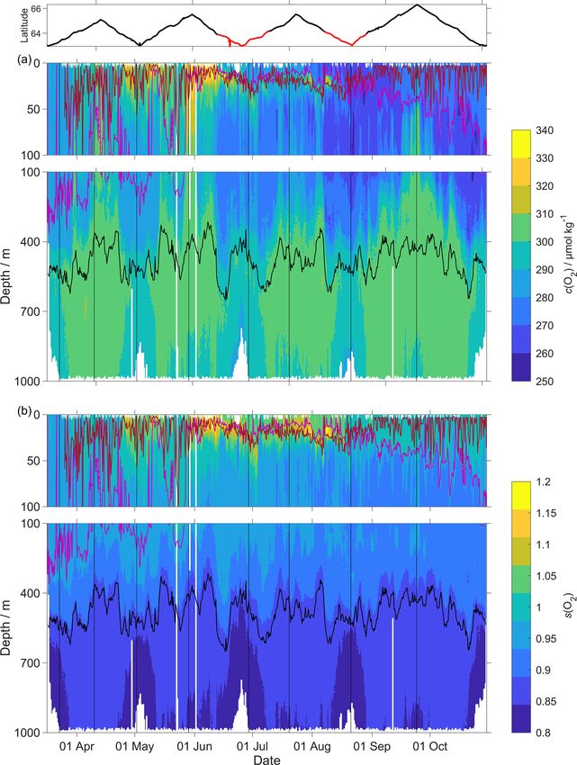
594                L. Possenti et al.: Norwegian Sea net community production from O2 and CO2 optode measurements

has taken up approximately 25 % of this anthropogenic CO2          cific depth that is commonly defined relative to the mixed
with a rate of (2.5 ± 0.6) Gt a−1 (in C equivalents) (Friedling-   layer depth (zmix ) or the bottom of the euphotic zone (Plant
stein et al., 2019). This uptake alters the carbonate system of    et al., 2016). A system is defined as autotrophic when GPP
seawater and is causing a decrease in seawater pH, a process       is larger than CR (i.e. NCP is positive) and as heterotrophic
known as ocean acidification (Gattuso and Hansson, 2011).          when CR is larger than GPP (i.e. NCP is negative) (Ducklow
The processes affecting the marine carbonate system include        and Doney, 2013).
air–sea gas exchange, photosynthesis and respiration, advec-          NCP can be quantified using bottle incubations or in situ
tion and vertical mixing, and CaCO3 formation and dissolu-         biogeochemical budgets (Sharples et al., 2006; Quay, et al,
tion. For that reason, it is important to develop precise, ac-     2012; Seguro et al., 2019). Bottle incubations involve mea-
curate and cost-effective tools to observe CO2 trends, vari-       suring production and respiration in vitro under dark and
ability and related processes in the ocean. Provided that suit-    light conditions. Biogeochemical budgets combine O2 and
able sensors are available, autonomous ocean glider mea-           DIC inventory changes with estimates of air–sea gas ex-
surements may help resolve these processes.                        change, entrainment, advection and vertical mixing (Neuer
   To quantify the marine carbonate system, four variables         et al., 2007; Alkire et al., 2014; Binetti et al., 2020).
are commonly measured: total dissolved inorganic car-                 The Norwegian Sea is a complex environment due to the
bon concentration, c(DIC); total alkalinity, AT ; the fugac-       interaction between the Norwegian Atlantic Current (NwAC)
ity of CO2 , f (CO2 ); and pH. At thermodynamic equilib-           entering from the south-west, Arctic Water coming from the
rium, knowledge of two of the four variables is sufficient         north and the Norwegian Coastal Current (NCC) flowing
to calculate the other two. Marine carbonate system vari-          along the Norwegian coast (Nilsen and Falck, 2006). In par-
ables are primarily measured on research ships, commercial         ticular, Atlantic Water enters the Norwegian Sea through the
ships of opportunity, moorings, buoys and floats (Hardman-         Faroe–Shetland Channel and Iceland–Faroe Ridge (Hansen
Mountford et al., 2008; Monteiro et al., 2009; Takahashi et        and Østerhus, 2000) with salinity S between 35.1 and 35.3
al., 2009; Olsen et al., 2016; Bushinsky et al., 2019). Moor-      and temperatures (θ ) warmer than 6 ◦ C (Swift, 1986). The
ings equipped with submersible sensors often provide limited       NCC water differs from the NwAC with a surface S < 35
vertical and horizontal but good long-term temporal resolu-        (Saetre and Ljoen, 1972) and a seasonal θ signal (Nilsen and
tion (Hemsley, 2003). In contrast, ship-based surveys have         Falck, 2006).
higher vertical and spatial resolution than moorings but lim-         Biological production in the Norwegian Sea varies dur-
ited repetition frequency because of the expense of ship op-       ing the year and five different periods can be discerned
erations. Ocean gliders have the potential to replace some         (Rey, 2004): (1) winter with the smallest productivity and
ship surveys because they are much cheaper to operate and          phytoplankton biomass; (2) a pre-bloom period; (3) the
will increase our coastal and regional observational capacity.     spring bloom when productivity increases and phytoplank-
However, the slow glider speed of 1–2 km h−1 only allows a         ton biomass reaches the annual maximum; (4) a post-bloom
smaller spatial coverage than ship surveys, and the sensors        period with productivity mostly based on regenerated nutri-
require careful calibration to match the quality of data pro-      ents; (5) autumn with smaller blooms than in summer. Pre-
vided by ship-based sampling.                                      vious estimates of the DIC-based net community production
   Carbonate system sensors suitable for autonomous deploy-        (N(DIC)) were based on discrete c(DIC) samples (Falck and
ment have been developed in the past decades, in particular        Anderson, 2005) or calculated from c(O2 ) measurements and
pH sensors (Seidel et al., 2008; Martz et al., 2010; Rérolle       converted to C equivalents assuming Redfield stoichiometry
et al., 2013) and p(CO2 ) sensors (Atamanchuk et al., 2014;        of production or respiration (Falck and Gade, 1999; Skjel-
Bittig et al., 2012; Degrandpre, 1993; Goyet et al., 1992;         van et al., 2001; Kivimäe, 2007). Glider measurements have
Körtzinger et al., 1996). One of these sensors is the CO2 op-      been used to estimate NCP in other ocean regions (Nichol-
tode (Atamanchuk et al., 2014), which has been successfully        son et al., 2008; Alkire et al., 2014; Haskell et al., 2019; Bi-
deployed to monitor an artificial CO2 leak on the Scottish         netti et al., 2020); however, as far as we know, this is the first
west coast (Atamanchuk, et al., 2015b), on a cabled under-         study of net community production in the Norwegian Sea us-
water observatory (Atamanchuk et al., 2015a), to measure           ing a high-resolution glider dataset (> 106 data points; 40 s
lake metabolism (Peeters et al., 2016), for fish transportation    time resolution) and the first anywhere estimating NCP from
(Thomas et al., 2017) and on a moored profiler (Chu et al.,        a glider-mounted sensor directly measuring the marine car-
2020).                                                             bonate system.
   c(DIC) and c(O2 ) measurements can be used to calcu-
late net community production (NCP), which is defined as
the difference between gross primary production (GPP) and
community respiration (CR). At steady state, NCP is equal
to the rate of organic carbon export and transfer from the
surface into the mesopelagic and deep waters (Lockwood et
al., 2012). NCP is derived by vertical integration to a spe-

Ocean Sci., 17, 593–614, 2021                                                           https://doi.org/10.5194/os-17-593-2021
L. Possenti et al.: Norwegian Sea net community production from O2 and CO2 optode measurements                                   595

Table 1. Average sampling interval of Sea-Bird CTD, Aanderaa          1000 m) were collected on five different cruises on the
4330F oxygen optode, Aanderaa 4797 CO2 optode and a combined          R/V Haakon Mosby along the southern half of the glider
backscatter/chlorophyll a fluorescence sensor (Wetlabs Eco Puck       transect on 18 March, 5 May, 6 and 14 June, and 30 Octo-
BB2FLVMT) in the top 100, from 100 to 500 and from 500 to             ber 2014. Samples for c(DIC) and AT were collected from
1000 m.                                                               10 L Niskin bottles following standard operational procedure
                                                                      (SOP) 1 of Dickson et al. (2007). The c(DIC) and AT samples
    Depth/m       t(CTD)/s     t(O2 )/s   t(CO2 )/s   t(Chl a)/s
                                                                      were preserved with saturated HgCl2 solution (final HgCl2
    0–100 m              24        49          106           62       concentration: 15 mg dm−3 ) and analysed within 14 d after
    100–500 m            31       153          233            –       the collection. Nutrient samples from the same Niskin bottles
    500–1000 m           42       378          381            –       were preserved with chloroform (Hagebo and Rey, 1984).
                                                                      c(DIC) and AT were analysed on shore according to SOPs 2
                                                                      and 3b (Dickson et al., 2007) using a VINDTA 3D (Mar-
                                                                      ianda) with a CM5011 coulometer (UIC instruments) and a
                                                                      VINDTA 3S (Marianda), respectively. The precision of the
                                                                      samples’ c(DIC) and AT values was 1 µmol kg−1 for both,
                                                                      based on duplicate samples and running Certified Reference
                                                                      Material (CRM) batch numbers 118 and 138 provided by
                                                                      professor A. Dickson, Scripps Institution of Oceanography,
                                                                      San Diego, USA (Dickson et al., 2003). Nutrients were anal-
                                                                      ysed on shore using an Alpkem AutoAnalyzer. In addition,
                                                                      43 water samples were collected at Ocean Weather Station M
                                                                      (OWSM) on five different cruises: 22 March on R/V Haakon
                                                                      Mosby, 9 May on R/V G.O. Sars, 14 June on R/V Haakon
                                                                      Mosby, 2 August and 13 November 2014 on R/V Johan Hjort
                                                                      from 10, 30, 50, 100, 200, 500, 800 and 1000 m depths.
Figure 1. Map of the glider deployment and the main currents.         The OWSM samples were preserved and analysed for AT
The black dots are the glider dives; the green and the red dots are   and c(DIC) as the Svinøy samples. No phosphate and sil-
the water samples collected along the glider section and at Ocean
                                                                      icate samples were collected at OWSM. Temperature (θ )
Weather Station M (OWSM), respectively. The three main water
masses (Skjelvan et al., 2008) are the Norwegian Coastal Current
                                                                      and salinity (S) profiles were measured at each station us-
(yellow), the Norwegian Atlantic Current (NwAC, orange) and Arc-      ing a Sea-Bird 911 plus CTD. pH and f (CO2 ) were cal-
tic Water (green).                                                    culated using the MATLAB toolbox CO2SYS (Van Heuven
                                                                      et al., 2011), with the following constants: K1 and K2 car-
                                                                      bonic acid dissociation constants of Lueker et al. (2000),
                                                                                     2−
2     Materials and methods                                           K(HSO−   4 /SO4 ) bisulfate dissociation constant of Dickson
                                                                      (1990) and borate to chlorinity ratio of Lee et al. (2010). The
2.1    Glider sampling                                                precision of AT and c(DIC) led to an uncertainty in the calcu-
                                                                      lated c(CO2 ) of 0.28 µmol kg−1 . For the OWSM calculations,
Kongsberg Seaglider 564 was deployed in the Norwegian                 we used nutrient concentrations from the Svinøy section at a
Sea on 16 March 2014 at 63.00◦ N, 3.86◦ E, and recovered              time as close as possible to the OWSM sampling as input.
on 30 October 2014 at 62.99◦ N, 3.89◦ E. The Seaglider                In the case of the glider, we derived a parameterisation for
was equipped with a prototype Aanderaa 4797 CO2 optode,               phosphate and silicate concentration as a function of sam-
an Aanderaa 4330F oxygen optode (Tengberg et al., 2006),              ple depth and time. This parameterisation had an uncertainty
a Sea-Bird conductivity–temperature–depth profiler (CTD)              of 1.3 and 0.13 µmol kg−1 and a R 2 of 0.6 and 0.4, for sili-
and a combined backscatter–chlorophyll a fluorescence sen-            cate and phosphate concentrations, respectively. The uncer-
sor (Wetlabs Eco Puck BB2FLVMT). The mean sampling                    tainty was calculated as the root mean square difference be-
intervals for each sensor varied with depth (Table 1).                tween measured and parameterised concentrations. This nu-
   The deployment followed the Svinøy trench from the                 trient concentration uncertainty contributed an uncertainty of
open sea towards the Norwegian coast. The glider covered              0.04 µmol kg−1 in the calculation of c(CO2 ), which is neg-
a 536 km long transect eight times (four times in each direc-         ligible and smaller than the uncertainty caused by AT and
tion) for a total of 703 dives (Fig. 1).                              c(DIC).

2.2    Discrete sampling                                              2.3   Oxygen optode calibration

During the glider deployment, 70 discrete water samples               The last oxygen optode calibration before the deployment
from various depths (5, 10, 20, 30, 50, 100, 300, 500 and             was performed in 2012 as a two-point calibration at 9.91 ◦ C

https://doi.org/10.5194/os-17-593-2021                                                              Ocean Sci., 17, 593–614, 2021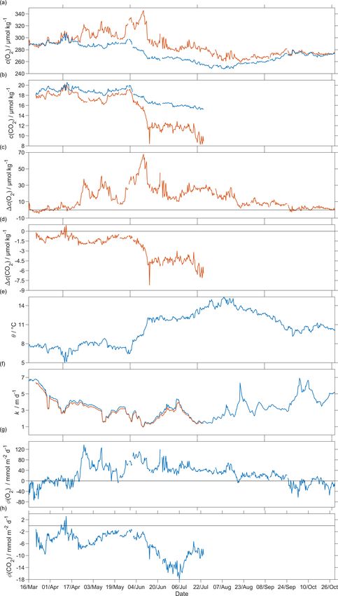
596                L. Possenti et al.: Norwegian Sea net community production from O2 and CO2 optode measurements

Figure 2. Glider oxygen concentration,            cG (O2 ),   for
σ0 > 1028 kg m−3 coloured by latitude.

in air-saturated water and at 20.37 ◦ C in anoxic Na2 SO3 solu-     Figure 3. A linear fit of the ratio between the daily median of the
tion. Oxygen optodes are known to be affected by drift (Bit-        discrete oxygen samples (cC (O2 )) and glider oxygen data (cG (O2 ))
                                                                    for σ0 > 1028 kg m−3 was used to derive the cG (O2 ) drift and ini-
tig and Körtzinger, 2015), which is even worse for the fast-
                                                                    tial offset at deployment. The time difference 1t is calculated with
response foils used in the 4330F optode for glider deploy-
                                                                    respect to the deployment day on 16 March.
ments. It has been suggested that it is necessary to calibrate
and drift correct the optode using discrete samples or in-air
measurements (Nicholson and Feen, 2017). Unfortunately,
no discrete samples were collected at glider deployment or          2.4   CO2 optode measurement principle
recovery.
   To overcome this problem, we used archived data to cor-          The CO2 optode consists of an optical and a temperature sen-
rect for oxygen optode drift. These archived concentration          sor incorporated into a pressure housing. The optical sensor
data (designated cC (O2 )) were collected at OWSM between           has a sensing foil comprising two fluorescence indicators (lu-
2001 and 2007 (downloaded from ICES database) and in the            minophores), one of which is sensitive to pH changes, and
glider deployment region between 2000 and 2018 (extracted           the other is not and thus used as a reference. The excitation
from GLODAPv2; Olsen et al., 2016). To apply the correc-            and emission spectra of the two fluorescence indicators over-
tion, we used the oxygen samples corresponding to a poten-          lap, but the reference indicator has a longer fluorescence life-
tial density σ0 > 1028 kg m−3 (corresponding to depths be-          time than the pH indicator. These two fluorescence lifetimes
tween 427 and 1000 m), because waters of these potential            are combined using an approach known as dual lifetime ref-
densities were always well below the mixed layer and there-         erencing (DLR) (Klimant et al., 2001; von Bültzingslöwen
fore subject to limited seasonal and interannual variability,       et al., 2002). From the phase shift (ϕ), the partial pressure
as evidenced by the salinity S and potential temperature θ of       of CO2 , p(CO2 ), is parameterised as an eight-degree poly-
these samples: S varied from 34.88 to 34.96, with a mean of         nomial (Atamanchuk et al., 2014):
34.90 ± 0.01; θ varied from 0.45 to −0.76 ◦ C, with a mean
of (−0.15 ± 0.36) ◦ C.                                              log[p(CO2 )/µatm] = C0 + C1 ϕ + . . . + C8 ϕ 8 ,                (1)
   Figure 2 shows that the glider oxygen concentration
(cG (O2 )) corresponding to σ0 > 1028 kg m−3 was charac-            where C0 to C8 are temperature-dependent coefficients.
terised by two different water masses separated at a latitude          The partial pressure of CO2 is linked to the CO2 concen-
of about 64◦ N. We used the samples collected north of 64◦ N        tration, c(CO2 ) and the fugacity of CO2 , f (CO2 ), via the fol-
to derive the glider optode correction because this reflects the    lowing relationship:
largest area covered by the glider. We did not use the south-
ern region because the archived samples from there covered
                                                                    c(CO2 ) = p(CO2 )/[1 − p(H2 O)/p]F (CO2 )
only 5 d. For each day of the year with archived samples,
we calculated the median concentration of the glider and the                 = K0 (CO2 )f (CO2 ),                                   (2)
archived samples. Figure 3 shows a plot of the ratio between
cC (O2 )/cG (O2 ) against the day of the year and a linear fit,     where F (CO2 ) is the solubility function (Weiss and Price,
which is used to calibrate cG (O2 ) and correct for drift.          1980), p(H2 O) is the water vapour pressure, p is the total
   No lag correction was applied because the O2 optode had          gas tension (assumed to be near 1 atm), and K0 (CO2 ) is the
a fast response foil and showed no detectable lag (< 10 s),         solubility coefficient. F and K0 vary according to tempera-
based on a comparison between descent and ascent profiles.          ture and salinity.

Ocean Sci., 17, 593–614, 2021                                                             https://doi.org/10.5194/os-17-593-2021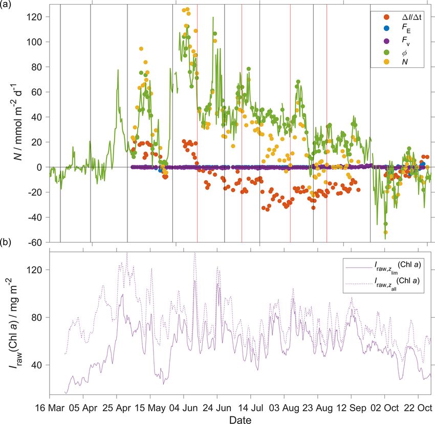
L. Possenti et al.: Norwegian Sea net community production from O2 and CO2 optode measurements                                       597

Figure 4. Panel (a) shows the calibrated p(CO2 ) (pcal (CO2 )) in       Figure 5. The histogram shows the distribution of the τ calculated
black and the discrete samples in azure. (b) Plot of p(CO2 ) ver-       from glider dives 31 to 400 to correct the CO2 optode drift using
sus depth where the continuous vertical lines are the mean every        the algorithm of Miloshevich (2004).
50 m and the error bars represent the standard deviation. Blue colour
shows pu (CO2 ) without any correction; red shows pd (CO2 ) cor-
rected for drift; green represents pc (CO2 ) corrected for drift and
                                                                        sponse time (τ ) and the ambient variability (Miloshevich,
lag; black shows pcal (CO2 ) calibrated against water samples (azure    2004). Before the lag correction, ϕcal,d was smoothed to re-
dots) collected during the deployment (Sect. 2.5). pcal (CO2 ) had      move any outliers and “kinks” in the profile using the Matlab
a mean standard deviation of 22 µatm and a mean bias of 1.8 µatm        function rLOWESS. The smoothing function applies a local
compared with the discrete samples.                                     regression every nine points using a weighted robust linear
                                                                        least-squares fit. Subsequently, τ was determined such that
                                                                        the following lag-correction equation (Miloshevich, 2004)
2.5   CO2 optode lag and drift correction and calibration               minimised the ϕcal,d difference between each glider ascent
                                                                        and the following descent:
The CO2 optode was fully functional between dives 31 (on
                                                                                         pd (CO2 , t1 ) − pd (CO2 , t0 )e−1t/τ
21 March 2014) and 400 (on 24 July 2014). After dive 400,               pc (CO2 t1 ) =                                         ,      (3)
the CO2 optode stopped sampling in the top 150 m. Fig-                                                1 − e−1t/τ
ure 4 shows the outcome of each calibration step: (0) un-               where pd (CO2 , t0 ) is the drift-corrected value measured by
calibrated optode output (blue dots), (1) drift correction (red         the optode at time t0 , pd (CO2 , t1 ) is the measured value
dots), (2) lag correction (green dots) and (3) calibration using        at time t1 , 1t is the time between t0 and t1 , τ is the re-
discrete water samples (black dots).                                    sponse time, and pc (CO2 , t1 ) is the lag-corrected value at
   In order to correct for the drift occurring during the glider        t1 . We calculated a τ value for each glider dive and used
mission, we selected the CO2 optode measurements in water               the median of τ (1384 s, 25th quartile: 1101 s; 75th quartile:
with σ0 > 1028 kg m−3 (just as for O2 ; Sect. 2.3). We calcu-           1799 s) (Fig. 5), which was larger than 1t(258 s) and there-
lated the median of the raw optode phase shift data (“Cal-              fore met the requirement to apply the Miloshevich (2004)
Phase” ϕcal ) for each Seaglider dive. Then, we calculated a            method. To apply the lag correction, the glider needs to sam-
drift coefficient (mi ) as the ratio between the median ϕcal for        ple same water mass during the ascent and descent. The dif-
a given dive divided by the median ϕcal of dive 31. Drift-              ference between the ascent and descent was minimal: it was
corrected ϕcal,d values were calculated by dividing the raw             (0.13 ± 0.33) ◦ C for θ and 0.02 ± 0.04 for S. This lag cor-
ϕcal by the specific mi for each dive.                                  rection reduced the average difference between glider ascent
   The CO2 optode was also affected by lag (Atamanchuk et               and descent from (71 ± 30) to (21 ± 26) µatm.
al., 2014) caused by the slow response of the optode to ambi-               The CO2 optode output was calibrated using the discrete
ent c(CO2 ) changes in time and depth. The lag created a dis-           samples collected throughout the mission. Using the discrete
crepancy between the depth profiles obtained during glider              sample time and potential density σ0 , we selected the clos-
ascents and descents. To correct for this lag, we applied the           est CO2 optode output. A linear regression between optode
method of Miloshevich (2004), which was previously used                 output and c(CO2 ) from the discrete samples (cWS (CO2 )
by Fiedler et al. (2013) and Atamanchuk et al. (2015b) to               was used to calibrate the optode output pc (CO2 ) in terms
correct the lag of the Contros HydroC CO2 sensor (Fiedler et            of c(CO2 ). c(CO2 ) had a better correlation than p(CO2 )
al., 2013; Saderne et al., 2013). This CO2 sensor has a dif-            (R 2 = 0.77 vs. R 2 = 0.02).
ferent measurement principle (infrared absorption) than the                 Plotting the regression residuals (cr (CO2 ), calculated as
CO2 optode, but both rely on the diffusion of CO2 through a             the difference between cWS (CO2 ) and the value predicted by
gas-permeable membrane.                                                 the regression) revealed a quadratic relation between the re-
   To apply the lag correction, the sampling interval (1t)              gression residuals and water temperature (θ). We have there-
needs to be sufficiently small compared to the sensor re-               fore included θ and θ 2 in the optode calibration (Fig. 6a).

https://doi.org/10.5194/os-17-593-2021                                                                    Ocean Sci., 17, 593–614, 2021
598                  L. Possenti et al.: Norwegian Sea net community production from O2 and CO2 optode measurements

                                                                        et al., 2016) data from the year 2000 in the deployment re-
                                                                        gion. Discrete samples with S < 33 were removed because
                                                                        these values were lower than the minimum S measured by
                                                                        the glider. The derived AT parameterisation is

                                                                        AT,reg /(µmol kg−1 ) = 2317.03 ± 12 + 33.12 ± 6.21(S − 35)
                                                                                           + 7.94 ± 11.38(S − 35)2
                                                                                           + 0.96 ± 1.79(θ/◦ C − 20)
                                                                                           + 0.01 ± 0.06(θ/◦ C − 20)2 .              (4)

                                                                        The parameterisation has an uncertainty of 8.2 µmol kg−1
                                                                        calculated as the standard deviation of the residual difference
                                                                        between actual and parameterised AT .
                                                                           To test this parameterisation, we compared the predicted
                                                                        AT,reg values with discrete measurements (AT,WS ) collected
                                                                        close in terms of time, potential density (σ0 ) and dis-
                                                                        tance to the glider transect (n = 60). These discrete sam-
                                                                        ples and the glider had mean temperature and salinity
                                                                        differences of (0.17 ± 0.68) ◦ C and 0.03 ± 0.013, respec-
                                                                        tively. The mean difference between AT,WS and AT,reg was
                                                                        (2.1 ± 6.5) µmol kg−1 .
                                                                           This AT parameterisation was used in CO2SYS (Van
                                                                        Heuven et al., 2011) to calculate c(DIC) from AT,reg and the
                                                                        calibrated c(CO2 ), cG,cal (CO2 ). These calculated cG,cal (DIC)
                                                                        values were compared with cWS (DIC) of the same set of dis-
                                                                        crete samples used to calibrate cG,cal (CO2 ), the only differ-
Figure 6. Regression (black lines, reg1) of the CO2 optode output       ence being that instead of the actual total alkalinity of the
pc (CO2 ) against (a) co-located concentration cWS (CO2 ) that has an   water sample (AT,WS ), we used AT,reg . The mean difference
uncertainty of 0.28 µmol kg−1 (b) and partial pressure pWS (CO2 )       between cG,cal (DIC) and cWS (DIC) was (3 ± 11) µmol kg−1 ,
of CO2 in discrete water samples (black dots). Also shown are the       with the non-zero bias and the standard deviation due to
values predicted by including θ and θ 2 in the regression used for      the uncertainties in the AT,reg parameterisation and the
optode calibration (red dots, reg2). The regression equations are       cG,cal (CO2 ) calibration.
(a) reg1: cWS (CO2 )/(µmol kg−1 ) = (0.033 ± 0.003)pc (CO2 )/µatm
– 1.8 ± 1.6 (R 2 = 0.77); reg2: cWS (CO2 )/(µmol kg−1 ) =               2.7   Quality control of other measurement variables
(0.12 ± 0.14)θ /◦ C – (0.071 ± 0.011)(θ /◦ C)2 + (0.0094 ±
0.0048)pc (CO2 )/µatm + 16 ± 4 (R 2 = 0.90). (b) reg1:                  The thermal lag of the glider conductivity sensor was cor-
pWS (CO2 )/µatm = (0.05 ± 0.05)pc (CO2 )/µatm + 344 ± 33                rected using the method of Gourcuff (2014). Single-point
(R 2 = 0.02); reg2: pWS (CO2 )/µatm = (21 ± 3)θ /◦ C – (1.9 ±           outliers in conductivity were removed and replaced by lin-
0.2)(θ /◦ C)2 + (0.2 ± 0.1)pc (CO2 )/µatm + 209 ± 76 (R 2 = 0.60).
                                                                        ear interpolation. The glider CTD salinity was affected by
                                                                        presumed particulate matter stuck in the conductivity cell
This second calibration increased the correlation coefficient           (Medeot et al., 2011) during dives 147, 234, 244, 251, 272,
R 2 from 0.77 to 0.90 and decreased the standard deviation              279, 303, 320 and 397, and sensor malfunction caused a poor
of the regression residuals from 1.3 to 0.8 µmol kg−1 . Even            match between glider ascent and descent during dives 214,
with the explicit inclusion of temperature in the calibration,          215, 235 and 243. These dives were removed from the sub-
the CO2 optode response remained more closely related to                sequent analysis.
c(CO2 ) than p(CO2 ) (Fig. 6b).                                            Glider-reported chlorophyll concentrations, craw (Chl a),
                                                                        were computed using the factory coefficients. craw (Chl a)
2.6   Regional algorithm to estimate AT                                 was affected by photochemical quenching during the day-
                                                                        time dives. To correct for quenching, we used the method
To calculate c(DIC), we used two variables: (1) glider                  of Hemsley et al. (2015) based on the nighttime relation-
c(CO2 ) derived as described in Sect. 2.5 and (2) AT derived            ship between fluorescence and optical backscatter. This re-
using a regional algorithm based on S and θ depths of less              lationship was established in the top 60 m and the nighttime
than 1000 m. The algorithm followed the approach of Lee                 values were selected between sunset and sunrise. We cal-
et al. (2006) and was derived using 663 water samples col-              culated a linear fit between craw (Chl a) measured at night,
lected at OWSM from 2004 to 2014 and GLODAPv2 (Olsen                    cN (Chl a), and the backscatter signal measured at night (bN ).

Ocean Sci., 17, 593–614, 2021                                                               https://doi.org/10.5194/os-17-593-2021
L. Possenti et al.: Norwegian Sea net community production from O2 and CO2 optode measurements                                              599

The slope and the intercept were then used to derive cor-          We followed the method of Woolf and Thorpe (1991) that
rected daytime cD (Chl a). The glider-reported chlorophyll         includes the effect of bubble equilibrium supersaturation in
concentration has not been calibrated against in situ sam-         the calculations:
ples and is not expected to be accurate, even after correc-
tion for quenching. However, it should give an indication of       Φ(O2 ) = kw (O2 ){(C(O2 ) − [1 + ∆bub (O2 )]Csat (O2 )},                  (7)
the depth of the deep chlorophyll concentration maximum
(zDCM ) and the direction of chlorophyll concentration change      where kw (O2 ) is the gas transfer coefficient, ∆bub (O2 ) is the
(up/down). The 8 d means of craw (Chl a) were compared with        increase of equilibrium saturation due to bubble injection,
satellite 8 d composite chlorophyll concentration (Fig. 7)         and Csat (O2 ) is the oxygen saturation. Csat (O2 ) was calcu-
from Ocean Colour CCI (https://esa-oceancolour-cci.org/,           lated from S and θ using the solubility coefficients of Benson
last access: 7 May 2020) and gave a mean difference of             and Krause (1984), as fitted by Garcia and Gordon (1992).
(0.12 ± 0.08) mg m−3 .                                             ∆bub (O2 ) was calculated from the following equation:
                                                                                             2
2.8   Calculation of oxygen-based net community                                      U
                                                                   ∆bub (O2 ) = 0.01               ,                                         (8)
      production N (O2 )                                                             U0

Calculating net community production N from glider data is         where U is 10 m wind speed with 1 h resolution (ECMWF
challenging because the glider continuously moves through          ERA5;            https://www.ecmwf.int/en/forecasts/datasets/
different water masses. For that reason, we subdivided the         reanalysis-datasets/era5, last access: 1 February 2021)
transect by binning the data into 0.1◦ latitude intervals to       and U0 represents the wind speed when the oxygen con-
derive O2 concentration changes every two transects. The           centration is 1 % supersaturated and has a value of 9 m s−1
changes were calculated between transects in the same di-          (Woolf and Thorpe, 1991). U has a spatial resolution of
rection of glider travel (e.g. transects 1 and 3, both in the N–   0.25◦ latitude and 0.25◦ longitude and was interpolated to
S direction) to have approximately the same time difference        the glider position at the beginning of the dive.
(40–58 d) at every latitude. If instead we had used two con-          The transfer velocity kw (O2 ) was calculated based on
secutive transects, this would lead to a highly variable time      Wanninkhof (2014):
difference of near 0 to about 50 d along the transect.                                                     2
   We calculated N(O2 ) (in mmol m−2 d−1 ) from the oxy-                              Sc(O2 ) −0.5

                                                                   kw (O2 )                           U
                                                                            = 0.251                           .                              (9)
gen inventory changes (1I (O2 )/1t) corrected for air–sea          cm h−1              660           m s−1
exchange Φ(O2 ), normalised to zmix when zmix was deeper
than the integration depth of zlim , entrainment E(O2 ) and di-    The Schmidt number, Sc(O2 ), was calculated using the pa-
apycnal eddy diffusion Fv (O2 ):                                   rameterisation of Wanninkhof (2014). To account for wind
                                                                   speed variability, kw (O2 ) applied to calculate N(O2 ) was a
         1I (O2 )           min (zlim , zmix )                     weighted mean. This value was calculated using the varying
N(O2 ) =          + Φ(O2 )
           1t                    zmix                              daily-mean wind speed U in the time interval between tn and
       − E(O2 ) − Fv (O2 ).                                 (5)    tn+1 (1t) (50 d) using a five-point-median zmix (Sect. 3.2)
                                                                   (Reuer et al., 2007). The time interval is the same as the one
The inventory changes were calculated as the difference be-        used to calculate 1I1t(O2 )
                                                                                               .
tween two transects of the integrated oxygen concentration            The entrainment flux, E(O2 ), was calculated as the oxy-
C(O2 ). C(O2 ) (in mmol m−3 ) was derived from the oxygen          gen flux when the mixed layer depth deepens in time and is
content c(O2 ) (in µmol kg−1 ) by multiplication with the wa-      greater than zlim at time t2 :
ter density (about 1027 kg m−3 , but we used the actual val-
                                                                                                        zlim
ues). A default integration depth of 45 m was chosen to cap-                  I (O2 , t1 , zmix (t2 )) zmix(t )
                                                                                                                − I (O2 , t1 , zlim )
                                                                                                             2
ture the deepest extent of the deep chlorophyll maximum            E(O2 ) =                                                             ,   (10)
                                                                                                       t2 − t1
(zDCM ) found during the deployment, which likely represents
the extent of the euphotic zone.                                   where t2 − t1 represents the change in time, zmix is the mixed
   The inventory changes for every latitude bin were calcu-        layer depth, I (O2 , t1 , zmix (t2 )) is the expected inventory that
lated using the following equation:                                would result from a mixed layer deepening to zmix (t2 ) be-
             R 45 m                   R 45 m                       tween t2 and t1 , and I (O2 , t1 , zlim ) is the original inventory at
1I (O2 )      0     Cn+1 (O2 , z)dz − 0 Cn (O2 , z)dz              t1 .
          =                                           , (6)
   1t                          tn+1 − tn                                The effect of diapycnal eddy diffusion (Fv ) was calculated
                                                                   at zmix when it was deeper than zlim and at zlim when zmix
where n is the transect number, t is the day of the year, and
                                                                   was shallower than zlim , using the following equation:
C(O2 , z) is the vertical O2 concentration profile.
   The air–sea flux of oxygen, Φ(O2 ), was calculated for each                     ∂C(O2 )
glider dive using the median C(O2 ), θ and S in the top 10 m.      Fv (O2 ) = Kz           ,                                                (11)
                                                                                     ∂z

https://doi.org/10.5194/os-17-593-2021                                                                  Ocean Sci., 17, 593–614, 2021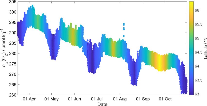
600                L. Possenti et al.: Norwegian Sea net community production from O2 and CO2 optode measurements

Figure 7. Comparison between the 8 d glider c(Chl a) (cG (Chl a)) mean and the 8 d satellite c(Chl a) (cS (Chl a)) download from Ocean
Colour CCI (https://esa-oceancolour-cci.org/, last access: 7 May 2020) as a time series (a) and scatter plot (b).

for a vertical eddy diffusivity (Kz ) of 10−5 m2 s−1                 descent of the following dive C(CO2 ). From this, Φ(CO2 )
(Naveira Garabato et al., 2004). The effect of Fv (O2 )              was calculated:
on N(O2 ) was negligible (Fig. A2b) with a median of
(−0.1 ± 0.5) mmol m−2 d−1 .                                          Φ(CO2 ) = k(CO2 )[C(CO2 ) − Catm (CO2 )].                                 (14)
                                                                     k(CO2 ) was calculated using the parameterisation of Wan-
2.9   Calculation of dissolved inorganic carbon-based
                                                                     ninkhof (2014):
      net community production, N (DIC)
                                                                                                               2
                                                                                         Sc(CO2 ) −0.5

                                                                     kw (CO2 )                            U
N(DIC) was expressed in mmol m−2 d−1 and was calculated                        = 0.251                            .        (15)
                                                                      cm h−1               660           m s−1
from DIC inventory changes (1I (DIC)/1t), air–sea flux of
CO2 , Φ(CO2 ), entrainment E(DIC) and diapycnal diffusion            Sc(CO2 ) is the dimensionless Schmidt number at the sea-
Fv (DIC):                                                            water temperature (Wanninkhof, 2014). To account for wind
                                                                     speed variability, kw (CO2 ) applied to calculate N(DIC) was a
             1(DIC)             min (zlim , zmix )
N (DIC) = −          − Φ (CO2 )                                      weighted mean based on the varying daily-mean wind speed
               1t                    zmix                            U in the time interval between tn and tn+1 (1t) used to calcu-
         + E (DIC) + Fv (DIC).                             (12)      late 1I 1t
                                                                             (DIC)
                                                                                   and for 40–50 d to calculate Φ(CO2 ) (Sect. 3.2)
                                                                     (Reuer et al., 2007).
Firstly, Φ(CO2 ) was calculated using the 10 m wind speed
                                                                        The DIC inventory changes were calculated in the top
with 1 h resolution downloaded from ECMWF ERA5. As
                                                                     45 m with the following equation:
for oxygen, we selected the closest wind speed data point
                                                                                   R 45 m                     R 45 m
at the beginning of each glider dive. We used the monthly            1I (DIC)               Cn+1 (DIC, z)dz − 0 Cn (DIC, z)dz
                                                                                    0
mean atmospheric CO2 dry mole fraction (x(CO2 )) down-                        =                                               . (16)
                                                                        1t                             tn+1 − tn
loaded from the Greenhouse Gases Reference Network Site
(https://www.esrl.noaa.gov/gmd/ccgg/ggrn.php, last access:           Just as for C(O2 ), C(DIC) (in mmol m−3 ) was derived from
28 February 2019) closest to the deployment at Mace Head,            the DIC content c(DIC) (in µmol kg−1 ) by multiplication
County Galway, Ireland (Dlugokencky et al., 2015). Us-               with the water density (about 1027 kg m−3 , but we used the
ing x(CO2 ), we calculated the air-saturation concentration          actual values).
Catm (CO2 ):                                                            The entrainment flux, E(DIC), was calculated as the DIC
                                                                     flux when the mixed layer depth deepens in time and is
Catm (CO2 ) = x(CO2 )pbaro F (CO2 ),                       (13)      greater than zlim at time t2 :
where pbaro is the mean sea level pressure and F (CO2 ) is                                                 zlim
                                                                                 I (DIC, t1 , zmix (t2 )) zmix(t   − I (DIC, t1 , zlim )
the CO2 solubility function (in mol dm−3 atm−1 ) calculated          E (DIC) =                                 2 )
                                                                                                                                           .   (17)
from surface θ and S (Weiss and Price, 1980).                                                           t2 − t1
   The seawater C(CO2 ) at the surface was calculated using          As for oxygen, the effect of diapycnal eddy diffusion (Fv )
the median in the top 10 m between the glider ascent and             was calculated at zmix when it was deeper than zlim and at

Ocean Sci., 17, 593–614, 2021                                                                https://doi.org/10.5194/os-17-593-2021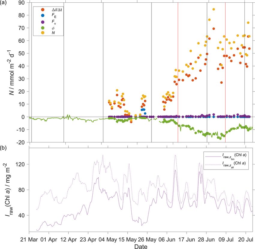
L. Possenti et al.: Norwegian Sea net community production from O2 and CO2 optode measurements                                     601

zlim when zmix was shallower than zlim , using the following
equation:
                ∂C(DIC)
Fv (DIC) = Kz           ,                                 (18)
                  ∂z
for a Kz of 10−5 m2 s−1 (Naveira Garabato et al., 2004). The
effect of Fv (DIC) was negligible (Fig. A2a) with a median of
(0.1 ± 0.3) mmol m−2 d−1 .
   The contribution of horizontal advection to N(DIC) was
considered minimal over the timescales where we calculated
inventory changes because previous studies have shown that
changes in C(DIC) during summer are mainly controlled by
biology and air–sea interactions (Gislefoss et al., 1998). For
that reason, previous studies that estimated N in the Norwe-
gian Sea have also neglected advective fluxes (Falck and An-
derson, 2005; Falck and Gade, 1999; Kivimäe, 2007; Skjel-
van et al., 2001).
   Uncertainties in N(DIC) and N(O2 ) were evaluated with
a Monte Carlo approach. The uncertainties of the input
variables are shown in Table 2; we repeated the analysis
1000 times. The total uncertainty in N was calculated as the
standard deviation of the 1000 Monte Carlo simulations.

3     Results

The uncorrected p(CO2 ) values presented in Fig. 8 were
analysed up to dive 400 (24 July 2014). For the following
dives, the CO2 optode stopped sampling in the first 150 m
(Fig. 8d). Instead, the uncorrected temperature θ , salinity S,
c(O2 ) and craw (Chl a) were analysed for all the dives (30 Oc-
tober 2014). The raw optode c(O2 ) data were calibrated and
drift corrected, and c(CO2 ) was drift corrected, lag corrected
and recalibrated, then used to quantify the temporal and spa-
tial changes in N and Φ together with the quenching cor-
rected craw (Chl a) to evaluate net community production
changes.                                                          Figure 8. Raw glider data for all 703 dives with latitude of the
                                                                  glider trajectory at the top (black: NwAC; red: NCC, separated by
3.1    O2 and CO2 optode calibration                              a S of 35). (a) Temperature θ , (b) salinity S, (c) oxygen concen-
                                                                  tration cG (O2 ), (d) uncorrected CO2 optode output pu (CO2 ) and
The O2 optode drift caused a continuous and unex-                 (e) chlorophyll a concentration craw (Chl a). The white space means
pected decrease of the uncorrected cG (O2 ) from 290 to           that the sensors did not measure any data. The pink line is zmix cal-
282 µmol kg−1 for σ0 > 1028 kg m−3 (Fig. 8c). The ratio           culated using a threshold criterion of 1θ = 0.5 ◦ C to the median θ
cC (O2 )/cG (O2 ) against day of the year used for the drift      in the top 5 m (Obata et al., 1996; Monterey and Levitus, 1997; Foltz
correction had a good correlation with time (R 2 = 0.90),         et al., 2003). The dotted black line designates zlim , used as a depth
showing a continuous increase of 0.0004 d−1 (Fig. 3), equiv-      limit to calculate N. Contoured black lines represent isopycnals.
alent to a decrease in the measured glider O2 concen-
tration of 0.11 µmol kg−1 d−1 . It was possible to apply
the correction because cC (O2 ) had low temporal variabil-           Following drift, lag and scale corrections, glider fugac-
ity for the chosen potential density σ0 > 1028 kg m−3 . The       ity fG (CO2 ) derived from Eq. (2) had a mean difference of
cC (O2 ) values from OWSM and GLODAPv2 had a mean                 (2 ± 22) µatm to the discrete samples (n = 55; not shown)
of (305 ± 3) µmol kg−1 , varying from 294 to 315 µmol kg−1        and c(DIC) had a mean difference of (3 ± 11) µmol kg−1
(Fig. A1). The drift correction reduced the variability of        (Fig. 10). p(CO2 ) and f (CO2 ) are almost identical, but
cG (O2 ) in the selected potential density range from a stan-     f (CO2 ) takes into account the non-ideal nature of the gas
dard deviation of 7.3 µmol kg−1 to a standard deviation of        phase. The optode was able to capture the temporal and spa-
2.4 µmol kg−1 (Fig. 9a).                                          tial variability showing that NCC had a lower DIC concentra-

https://doi.org/10.5194/os-17-593-2021                                                             Ocean Sci., 17, 593–614, 2021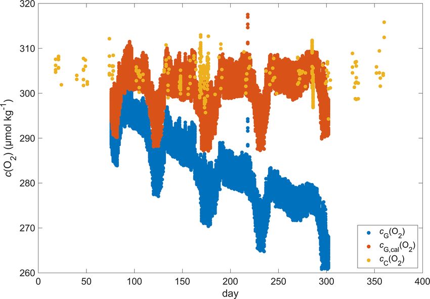
602 L. Possenti et al.: Norwegian Sea net community production from O2 and CO2 optode measurements
Table 2. Uncertainty associated with N (DIC) and N(O2 ) input variables calculated by a Monte Carlo approach.
Variable Error Reference/method
c(DIC) 11 µmol kg−1 Standard deviation of the differences to discrete water samples
S 0.01 Standard deviation of glider salinities for σ0 > 1028 kg m−3 and latitude > 64◦ N
θ 0.3 ◦ C Standard deviation of glider temperature for σ0 > 1028 kg m−3 and latitude > 64◦ N
Catm (CO2 ) 1.5 mmol m−3 Standard deviation of Catm (CO2 )
C(CO2 ) 0.8 mmol m−3 Standard deviation of the differences to discrete water samples
kw (CO2 ), kw (O2 ) 20 % Wanninkhof (2014)
zmix 9m Standard deviation for zmix based on thresholds 1T = 0.1 ◦ C (Sprintall and Roemmich, 1999),
0.2 ◦ C (Thompson, 1976) and 0.8 ◦ C (Kara et al., 2000)
c(O2 ) 2.4 µmol kg−1 Standard deviation of glider oxygen concentrations for σ0 > 1028 kg m−3 and latitude > 64◦ N
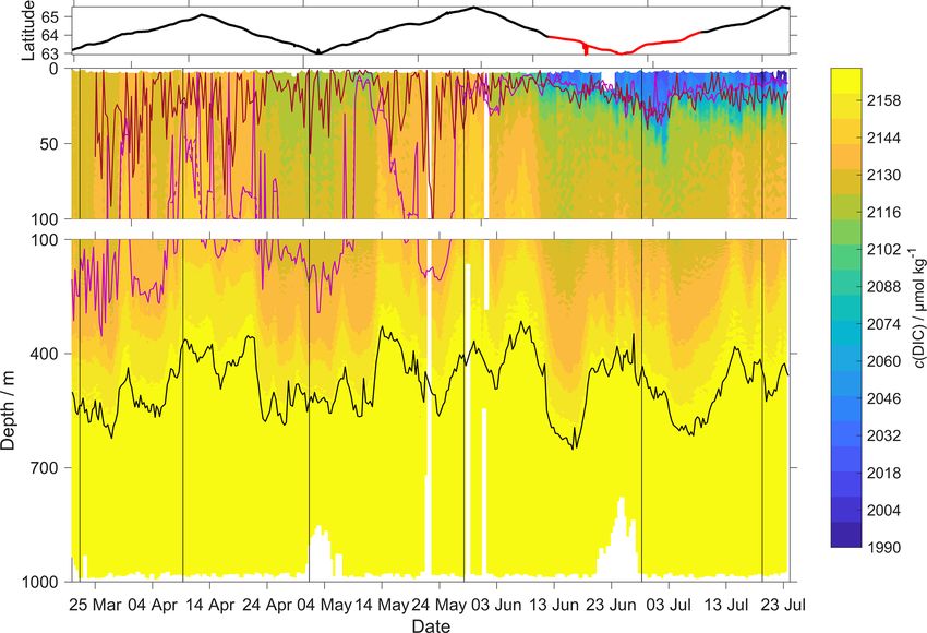
Figure 10. c(DIC) contour plot with zDCM (red line), zmix (pink
line) five-point median zmix (dotted pink line). The black line in-
dicates σ0 = 1028 kg m−3 . The top panel indicates glider latitude
(black: NwAC; red: NCC).
varied between 204 and 391 µatm, while fSOCAT (CO2 ) var-
ied between 202 and 428 µatm (Fig. 11).
Our results are in agreement with Jeansson et al. (2011),
who found the surface NCC was the region with the
lowest c(DIC) values (2083 µmol kg−1 ) in the Norwe-
gian Sea. This was confirmed during our deployment
because c(DIC) was (2081 ± 39) µmol kg−1 in the NCC
Figure 9. (a) c(O2 ); (b) s(O2 ) = c(O2 )/csat (O2 ) with zDCM (red region and (2146 ± 27) µmol kg−1 in the NwAC region
line), zmix (pink line) five-point median zmix (dotted pink line). (Fig. 10) and c(O2 ) was > 300 µmol kg−1 in the NwAC and
The black line indicates σ0 = 1028 kg m−3 . The top panel indicates < 280 µmol kg−1 in the NCC.
glider latitude (black: NwAC; red: NCC).
3.2 Air–sea exchange
tion than NwAC. Restricting the f (CO2 ) comparison to the The surface water was supersaturated with oxygen all sum-
discrete samples in the top 10 m gave a mean difference of mer (Fig. 12). From May, this supersaturation drove a con-
(19 ± 31) µatm (n = 6). We also compared glider fG (CO2 ) tinuous O2 flux from the sea to the atmosphere. However,
with the Surface Ocean CO2 Atlas (SOCAT) f (CO2 ) the flux varied throughout the deployment, having a median
(Bakker et al., 2016) data in the region during the deployment of 25 mmol m−2 d−1 (5th percentile: −31 mmol m−2 d−1 ;
(Fig. 11). During the whole deployment, there was general 95th percentile: 88 mmol m−2 d−1 ). Prior to the spring pe-
agreement between fG (CO2 ) and fSOCAT (CO2 ). fG (CO2 ) riod of increased Chl a inventory, the supersaturation var-
Ocean Sci., 17, 593–614, 2021 https://doi.org/10.5194/os-17-593-2021L. Possenti et al.: Norwegian Sea net community production from O2 and CO2 optode measurements 603
Figure 11. Comparison between surface f (CO2 ) from 2014 SO-
CAT and CO2 optode on the glider. (a) The black lines are the
median glider f (CO2 ) in the top 10 m, with fc (CO2 ) (dotted line)
corresponding to regression 1 (Fig. 6a) and ft (CO2 ) (continuous
line) to regression 2 (Fig. 6a). Discrete samples collected during
the deployment are shown as red dots, with the other coloured dots
representing cruises in the SOCAT database (Bakker et al., 2016).
(b) Glider and SOCAT data positions (same colours as in panel a).
ied between 0 to 10 µmol kg−1 . Φ(O2 ) had a median of
−1.4 mmol m−2 d−1 (5th percentile: −49 mmol m−2 d−1 ;
95th percentile: 23 mmol m−2 d−1 ). Then, during the spring
period of increased Chl a inventory, the surface concen-
tration increased by over 35 µmol kg−1 , causing a peak
in Φ(O2 ) of 140 mmol m−2 d−1 . A second period of in-
Figure 12. Air–sea flux of O2 and CO2 during spring and summer
creased Chl a inventory was encountered in June and had for CO2 and during spring, summer and autumn for O2 , (a) csat (O2 )
a larger Φ(O2 ) up to 118 mmol m−2 d−1 , driven by su- in blue and c(O2 ) in red, (b) csat (CO2 ) in blue and c(CO2 )
persaturation of 68 µmol kg−1 . The fluxes were smaller in red, (c) 1c(O2 ) = c(O2 ) − csat (O2 ), (d) 1c(CO2 ) = c(CO2 ) −
than during spring and were associated with an increase csat (CO2 ), (e) sea surface temperature, (f) kw (O2 ) in blue and
of craw (Chl a) from 2.5 mg m−3 to the summer maxi- kw (CO2 ) in red normalised back to 50 d (Reuer et al., 2007),
mum of 4.0 mg m−3 . However, prior to the increased spring (g) oxygen air–sea flux Φ(O2 ) and (h) CO2 air–sea flux Φ(CO2 ).
Chl a inventory, Φ(O2 ) showed a few days of influx The flux from sea to air is positive, while that from air to sea is
into seawater caused by a decrease of θ from 7.6 to negative.
5.9 ◦ C that increased Csat (O2 ). The influx at the begin-
ning of the deployment is partly due to the ∆bub (O2 ) cor-
rection that resulted in [1 + ∆bub (O2 )]csat (O2 ) > c(O2 ) for The CO2 flux from March to July was always
U > 10 m s−1 . In August, the surface supersaturation de- from the air to the sea (Fig. 12), with a median of
creased to 2.3 µmol kg−1 and Φ(O2 ) decreased to a monthly −5.2 mmol m−2 d−1 (5th percentile: −14 mmol m−2 d−1 ;
minimum of −7.6 mmol m−2 d−1 . In the second half of 95th percentile: −1.5 mmol m−2 d−1 ). An opposite flux di-
September, the surface water became undersaturated by rection is expected for Φ(O2 ) and Φ(CO2 ) during the
−2.6 µmol kg−1 , causing O2 uptake with a median flux productive season when net community production is the
of −13 mmol m−2 d−1 (5th percentile: −39 mmol m−2 d−1 ; main driver of concentration changes. After the summer pe-
95th percentile: 10 mmol m−2 d−1 ). riod of increased Chl a inventory, the flux had a median
https://doi.org/10.5194/os-17-593-2021 Ocean Sci., 17, 593–614, 2021604 L. Possenti et al.: Norwegian Sea net community production from O2 and CO2 optode measurements
of −11 mmol m−2 d−1 (5th percentile: −16 mmol m−2 d−1 ;
95th percentile: −6.8 mmol m−2 d−1 ), in agreement with
previous studies that classified the Norwegian Sea as a CO2
sink (Takahashi et al., 2002; Skjelvan et al., 2005). Φ(CO2 )
for the discrete samples from 18 March to 14 June (n = 13)
varied from 0.1 to −13 mmol m−2 d−1 .
3.3 N(O2 )
To capture the entire euphotic zone, we calculated N(O2 )
and N(DIC) using an integration depth of zlim = 45 m be-
cause the mean deep chlorophyll maximum (DCM) depth
was zDCM = (20 ± 18 m) (Fig. 9). For comparison, the mixed
layer depth was deeper, varied more strongly and had a mean
value of zmix = (68 ± 78) m, using a threshold criterion of
1θ = 0.5 ◦ C to the median θ value in the top 5 m of the glider
profile (Obata et al., 1996; Monterey and Levitus, 1997; Foltz
et al., 2003).
The two N values were calculated as the difference in
inventory changes between two transects when the glider
moved in the same direction. Figure 13. (a) Components of the N(O2 ) calculation: 1I (O2 )/1t
(red), E(O2 ) (blue), Fv (O2 ) (violet), Φ(O2 ) (green) with kw (O2 )
During the deployment, we sampled two periods of in-
weighted over 50 d, N(O2 ) (yellow). (b) Chl a inventory in the top
creased Chl a inventory, the first one in May and a second 45 m, Iraw,zlim (Chl a) (violet). Chl a inventory for the whole water
one in June. The chlorophyll a inventory (Iraw,zlim (Chl a)) column, Iraw,zall (Chl a) (dotted violet line). The vertical black lines
was calculated integrating craw (Chl a) to zlim . To remove out- represent each glider transect. Between the two vertical red lines,
liers, we used a five-point moving mean of Iraw,zlim (Chl a). the glider was in the NCC region.
The N(O2 ) changes were dominated by Φ(O2 ), which
had an absolute median of 34 mmol m−2 d−1 (5th percentile:
4.3 mmol m−2 d−1 ; 95th percentile: 86 mmol m−2 d−1 ), creasing to 27 mg m−2 leading to the minimum N(O2 ) of
followed by I (O2 ), which had a median of 15 mmol m−2 d−1 (−52 ± 11) mmol m−2 d−1 .
(5th percentile: 2.3 mmol m−2 d−1 ; 95th percentile: Integrating N (O2 ) from March to October gives a flux of
29 mmol m−2 d−1 ), Fv (O2 ), which had an absolute me- 4.9 mol m−2 a−1 (Table 3; discussed in Sect. 4.2).
dian of 0.3 mmol m−2 d−1 (5th percentile: 0 mmol m−2 d−1 ;
95th percentile: 1.0 mmol m−2 d−1 ) and E(O2 ), which 3.4 N(DIC)
had a median of 0 mmol m−2 d−1 (5th percentile:
−1.2 mmol m−2 d−1 ; 95th percentile: 0 mmol m−2 d−1 ). In the case of N(DIC), the main drivers were
At the beginning of May, Iraw,zlim (Chl a) increased the inventory changes with an absolute median of
to 97 mg m−2 and N(O2 ) = (95 ± 16) mmol m−2 d−1 . Af- 29 mmol m−2 d−1 (5th percentile: 1.3 mmol m−2 d−1 ;
ter this period, Iraw,zlim (Chl a) decreased to 49 mg m−2 95th percentile: 57 mmol m−2 d−1 ), followed by Φ(CO2 ),
and N (O2 ) = (−4.6 ± 1.6) mmol m−2 d−1 . During the sum- which had an absolute median of 7.0 mmol m−2 d−1
mer Iraw,zlim (Chl a) increased to 110 mg m−2 , which caused (5th percentile: 0.8 mmol m−2 d−1 ; 95th percentile:
a sharp increase of N(O2 ) to (126 ± 25) mmol m−2 d−1 . 15 mmol m−2 d−1 ), Fv (DIC), which had an absolute median
Iraw,zlim (Chl a) remained higher than 50 mg m−2 until the of 0.2 mmol m−2 d−1 (5th percentile: 0 mmol m−2 d−1 ;
end of June when N(O2 ) was (31 ± 9) mmol m−2 d−1 . The 95th percentile: 1.3 mmol m−2 d−1 ) and E(DIC), which
passage of the glider from NwAC to NCC was accompa- had a median of 0 mmol m−2 d−1 (5th percentile:
nied by a drop of surface c(O2 ) from 330 to 280 µmol kg−1 0 mmol m−2 d−1 ; 95th percentile: 3.4 mmol m−2 d−1 ).
(Fig. 9) that resulted in lower Φ(O2 ) and N(O2 ) values During the period of increased Chl a inventory N(DIC)
(Fig. 13). At the same time, Iraw,zlim (Chl a) decreased to was (21 ± 4.5) mmol m−2 d−1 . Later, Iraw,zlim (Chl a)
35 mg m−2 showing that the decrease of N(O2 ) depended decreased to 30 mg m−2 driving N(DIC) to negative
on the passage to NCC and a decrease of biological pro- values with a minimum of (−2.7 ± 5.0) mmol m−2 d−1 .
duction. After the beginning of August, Iraw,zlim (Chl a) de- In the next transect, the glider measured the maximum
creased to 49 mg m−2 and N(O2 ) turned negative with a Iraw,zlim (Chl a) of 111 mg m−2 that increased N(DIC) to
minimum of (−23 ± 25) mmol m−2 d−1 . In October, dur- (85 ± 4.5) mmol m−2 d−1 . This maximum was reached dur-
ing the last glider transect, Iraw,zlim (Chl a) continued de- ing a transect when the glider moved in NCC, which had a
Ocean Sci., 17, 593–614, 2021 https://doi.org/10.5194/os-17-593-2021L. Possenti et al.: Norwegian Sea net community production from O2 and CO2 optode measurements 605
a glider and was not actively pumped, which increased the
response time to 23 min (25th quartile: 18 min; 75th quartile:
30 min). Also, the optode was affected by a continuous drift
from 637 to 5500 µatm that was larger than the drift found by
Atamanchuk et al. (2015a) which increased by 75 µatm after
7 months.
In this study, the drift- and lag-corrected sensor out-
put showed a better correlation with the CO2 concentration
c(CO2 ) than with p(CO2 ). The latter two quantities are re-
lated to each other by the solubility that varies with θ and
S (Weiss, 1974) (Eq. 2). The better correlation with c(CO2 )
was probably related to an inadequate temperature parame-
terisation of the sensor calibration function. Including both
temperature and temperature squared in the calibration gave
a better fit with c(CO2 ) than with p(CO2 ) but overall still
a lower calibration residual for the former. The sensor out-
put depends on the changes in pH that are directly related
to the changes of c(CO2 ) in the membrane and – indirectly
– p(CO2 ), via Henry’s law. The calibration is supposed to
correct for the temperature dependence of the sensor output
(Atamanchuk et al., 2014). So the fact that the sensor output
Figure 14. (a) Components of the N(DIC) calculation: correlated better with c(CO2 ) than p(CO2 ) is perhaps due
1I (DIC)/1t (red), E(DIC) (blue), Fv (CO2 ) (violet), Φ(CO2 )
to a fortuitous cancellation of an inadequate temperature pa-
(green) with kw (CO2 ) weighted over 50 d, N (DIC) (yellow).
(b) Chl a inventory in the top 45 m, Iraw,zlim (Chl a) (violet). Chl a
rameterisation and Henry’s law relationship between c(CO2 )
inventory for the whole water column, Iraw,zall (Chl a) (dotted and p(CO2 ).
violet line). The vertical black lines represent each glider transect. The calibrated optode output captured the c(DIC) changes
Between the two vertical red lines, the glider was in the NCC in space and time with a standard deviation of 11 µmol kg−1
region. compared with the discrete samples. c(DIC) decreased
from 2130 to 2000 µmol kg−1 and increased with depth to
2170 µmol kg−1 . This shows the potential of the sensor for
c(DIC) of 2080 µmol kg−1 at the surface compared with the future studies that aim to analyse the carbon cycle using a
2150 µmol kg−1 in NwAC and drove a continuous positive high-resolution dataset.
N(DIC), which had a minimum of (36 ± 7.4) mmol m−2 d−1 The optode-derived CO2 fugacity fG (CO2 ) had a mean
(Fig. 14). bias of (1.8 ± 22) µatm compared with the discrete samples.
Integrating N(DIC) from March to July gives a flux of These values are comparable with a previous study when the
3.3 mol m−2 a−1 (Table 3; discussed in Sect. 4.2). CO2 optode was tested for 65 d on a wave-powered profil-
ing cRAWLER (PRAWLER) from 3 to 80 m (Chu et al.,
2020), which had an uncertainty between 35 and 72 µatm.
4 Discussion The PRAWLER optode was affected by a continuous drift of
5.5 µatm d−1 corrected using a regional empirical algorithm
4.1 Sensor performance that uses c(O2 ), θ , S and σo to estimate AT and c(DIC).
This study presents data from the first glider deployment with 4.2 Norwegian Sea net community production
a CO2 optode. The initial uncalibrated pu (CO2 ) measured
by the CO2 optode had a median of 604 µatm (5th percentile: Increases in N(O2 ) and N (DIC) were associated with in-
566 µatm; 95th percentile: 768 µatm), whereas the p(CO2 ) of creases in depth-integrated craw (Chl a), designated as peri-
discrete samples varied from 302 to 421 µatm. ods of increased Chl a inventory Iraw (Chl a), at the begin-
We applied corrections for drift (using deep-water samples ning of May and in June. During May, Iraw (Chl a) reached
as a reference point), sensor lag and calibrated the CO2 op- 135 mg m−2 . In June, Iraw (Chl a) reached again 135 mg m−2 .
tode against co-located discrete samples throughout the wa- Between these two periods, N(DIC) briefly turned negative,
ter column. indicating remineralisation of the high Chl a inventory ma-
Atamanchuk et al. (2014) reported that the sensor was af- terial during this period. The period of increased Chl a in-
fected by a lag that varied from 45 to 264 s depending on tem- ventory coincided with a surface temperature increase from
perature. These values were determined in an actively stirred 7 to 11 ◦ C and shoaling of the mixed layer from 200 to 20 m.
beaker. However, in this study, the sensor was mounted on c(O2 ) reached a summer maximum of 340 µmol kg−1 and
https://doi.org/10.5194/os-17-593-2021 Ocean Sci., 17, 593–614, 2021You can also read