Ice-shelf ocean boundary layer dynamics from large-eddy simulations
←
→
Page content transcription
If your browser does not render page correctly, please read the page content below
The Cryosphere, 16, 277–295, 2022
https://doi.org/10.5194/tc-16-277-2022
© Author(s) 2022. This work is distributed under
the Creative Commons Attribution 4.0 License.

Ice-shelf ocean boundary layer dynamics from large-eddy
simulations
Carolyn Branecky Begeman, Xylar Asay-Davis, and Luke Van Roekel
Theoretical Division, Los Alamos National Laboratory, P.O. Box 1663, Los Alamos, New Mexico 87545, USA

Correspondence: Carolyn Branecky Begeman (cbegeman@lanl.gov)

Received: 2 August 2021 – Discussion started: 1 September 2021
Revised: 27 November 2021 – Accepted: 6 December 2021 – Published: 24 January 2022

Abstract. Small-scale turbulent flow below ice shelves is        shelf base. Thus, accurate predictions of ice-shelf melting de-
regionally isolated and difficult to measure and simulate.       pend on representing the turbulent dynamics of the IOBL.
Yet these small-scale processes, which regulate heat and salt    This representation is also critical for evaluating the sensi-
transfer between the ocean and ice shelves, can affect sea-      tivity of the coupled land-ice–ocean system to changes in
level rise by altering the ability of Antarctic ice shelves to   ocean conditions. Of particular concern is the sensitivity of
“buttress” ice flux to the ocean. In this study, we improve      ice-shelf melting to increasing seawater temperature at depth,
our understanding of turbulence below ice shelves by means       a trend observed along a wide swath of the West Antarctic
of large-eddy simulations at sub-meter resolution, capturing     coastline and a potential trigger for West Antarctic Ice Sheet
boundary layer mixing at scales intermediate between lab-        collapse (Purkey et al., 2018; Ruan et al., 2021; Schmidtko
oratory experiments or direct numerical simulations and re-      et al., 2014; Wåhlin et al., 2021).
gional or global ocean circulation models. Our simulations          One indication that ocean models do not capture turbulent
feature the development of an ice-shelf ocean boundary layer     dynamics in the IOBL is that the simulated thermal driving,
through dynamic ice melting in a regime with low thermal         the difference between ocean temperature and the local freez-
driving, low ice-shelf basal slope, and strong shear driven by   ing point, and consequently the simulated melt rate differ sig-
the geostrophic flow. We present a preliminary assessment        nificantly between ocean models and as resolution is varied
of existing ice-shelf basal melt parameterizations adopted in    within a model (Gwyther et al., 2020). Furthermore, ocean
single component or coupled ice-sheet and ocean models on        models predict ice-shelf melting using parameterizations that
the basis of a small parameter study. While the parameter-       neglect the effects of the lateral buoyancy gradient of the
ized linear relationship between ice-shelf melt rate and far-    IOBL, and often of the vertical buoyancy gradient, on the
field ocean temperature appears to be robust, we point out       efficiency of vertical mixing near the boundary. This model
a little-considered relationship between ice-shelf basal slope   deficiency likely biases turbulent fluxes through the IOBL
and melting worthy of further study.                             and ocean cavity circulation, which is driven in large part by
                                                                 the buoyant flow of water freshened by ice-shelf melting, an
                                                                 overturning circulation also known as the “ice pump” (Web-
                                                                 ber et al., 2018). A new parameterization of ice-shelf melting
1   Introduction                                                 that accounts for the dynamics of IOBL turbulence is needed
                                                                 to achieve a more physically based, accurate coupling of ice
The largest source of uncertainty in future sea-level rise is    sheets and oceans in climate models (Dinniman et al., 2016;
the potential loss of ice from the Antarctic Ice Sheet (IPCC,    Edwards et al., 2021; Gwyther et al., 2020; Naughten et al.,
2014). The rate of grounded ice loss is highly sensitive to      2018). Supercooling of the IOBL and frazil ice accretion to
the melting of ice shelves, which drain over 80 % of Antarc-     the ice-shelf base are also regionally important processes for
tica’s grounded ice (Reese et al., 2018; Rignot et al., 2013).   cold cavities but are not the focus of this work (Galton-Fenzi
The ice-shelf ocean boundary layer (IOBL) controls ice-shelf     et al., 2012; Jordan et al., 2015).
melting by regulating oceanic heat and salt fluxes to the ice-

Published by Copernicus Publications on behalf of the European Geosciences Union.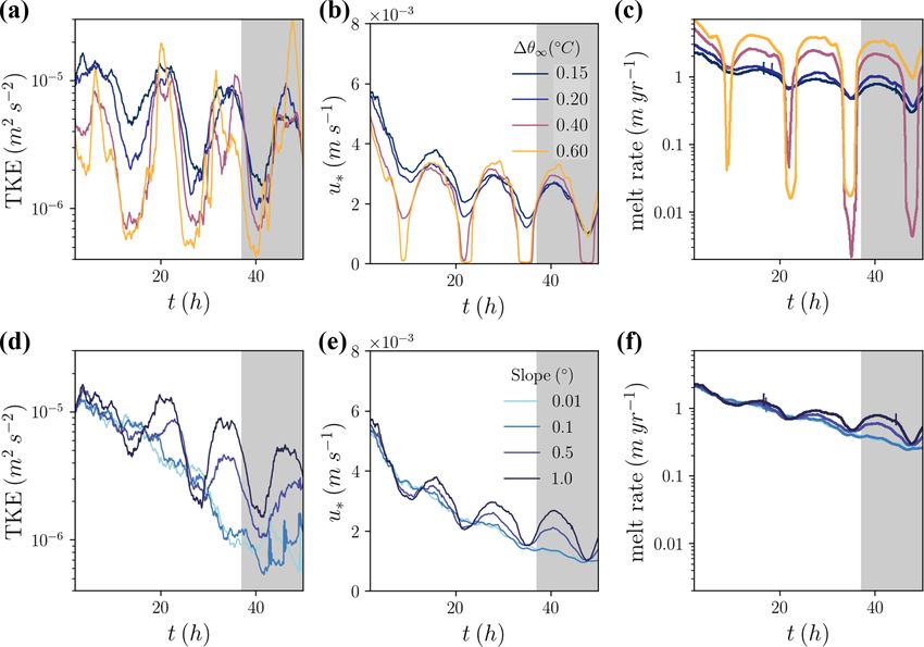
278                                                                                      C. B. Begeman et al.: IOBL dynamics

   IOBLs present unique conditions in the global ocean, in-        2     Methods
volving a stabilizing buoyancy flux from melting ice and a
boundary layer that is positively buoyant against a sloping        2.1    Overview of the LES model
boundary. There is a rich literature on stably stratified bound-
ary layers (typically under constant stabilizing flux boundary     The Parallelized Large-Eddy Simulation Model (PALM) was
conditions), but the dependence of heat, salt, and momentum        developed at the Institute of Meteorology and Climatol-
fluxes on stratification remains a difficult problem, especially   ogy at Leibniz University Hannover, Germany (Raasch and
for strongly stratified regimes (Zonta and Soldati, 2018).         Schröter, 2001), for simulation of atmospheric and ocean
IOBL turbulence has been explored through laboratory ex-           boundary layers. For this application to sub-ice-shelf set-
periments, direct numerical simulations, and large-eddy sim-       tings, we developed a new version based on PALM v5.0
ulations (Middleton et al., 2021; Mondal et al., 2019; Vreug-      (Maronga et al., 2015) with added features, including a
denhil and Taylor, 2019; McConnochie and Kerr, 2018; Ro-           boundary flux scheme for the ice–ocean interface, rotating
sevear et al., 2021). However, this body of work has not yet       the gravity and Coriolis vectors for sloped domains, and a
matured to setting a new standard for ice-shelf melt parame-       different turbulence closure scheme. Here, we provide a brief
terization in ocean models. Today, the most commonly used          overview of PALM with a focus on our additions. For more
ice-shelf melt parameterization is still derived from sea-ice      details we refer readers to Maronga et al. (2015).
conditions (i.e., in the absence of a slope), with some param-        The governing equations of PALM are the following:
eters tuned for ice-shelf settings (Holland and Jenkins, 1999;                                  ∂ui      ∂ui uj
Jenkins et al., 2010; McPhee et al., 1987). A knowledge gap        Momentum conservation            =−           − εij k fj uk
                                                                                                ∂t        ∂xj
exists in bridging IOBL dynamics across scales and charac-                                                               ρ − ρa
terizing the structure of buoyant plumes. Recently, this has                                        + εi3j f3 ug,j + gi
                                                                                                                            ρ0
been addressed through non-turbulence-resolving 2-d or 2.5-
                                                                                                       1 ∂π ∗       ∂
d models (Cheng et al., 2020; Jenkins, 2016, 2021). Notably,                                        −           −
Jenkins (2021) found that vertical mixing in IOBL settings                                            ρ0 ∂xi       ∂xj

was represented poorly by the commonly used K-profile pa-                                                00 00    1  00 00
                                                                                                    × ui uj − ui ui δij         , (1)
rameterization (KPP) in comparison to a higher-order turbu-                                                       3
lence closure scheme, suggesting that the application of KPP                             ∂uj
in ocean models may be inappropriate in ice-shelf cavities.        Volume conservation       = 0,                    (2)
                                                                                         ∂xj
   In this study, we model turbulent heat, salt, and momen-                           ∂θ      ∂uj θ    ∂  00 00
tum fluxes through the IOBL using large-eddy simulation            Heat conservation     =−         −     u θ + 8θ ,
                                                                                      ∂t       ∂xj    ∂xj j
(LES). Whereas the ocean models typically used to model
                                                                                                                     (3)
sub-ice-shelf circulation lack both the resolution and appro-
priate parameterizations needed to capture the relevant tur-                         ∂S      ∂uj S     ∂  00 00
                                                                   Salt conservation     =−         −     u S + 8S . (4)
bulent scales for boundary layer dynamics, LES captures the                          ∂t       ∂xj     ∂xj j
dominant energy-containing scales of turbulence and repre-            The momentum terms on the right hand side of Eq. (1) are,
sents smaller, unresolved scales with varying degrees of com-      in order, advection, Coriolis forcing, imposed geostrophic
plexity. An effective parameterization of ice-shelf melting is     flow with a geostrophic velocity ug , buoyancy forcing, a cor-
likely to rest on an understanding of how turbulent mixing         rection for divergence in the flow using the pressure perturba-
in the IOBL depends on stratification and shear forcing. We        tion π ∗ (imposing incompressibility), and sub-grid-scale mo-
vary far-field ocean temperature and ice-shelf slope between       mentum flux. All prognostic variables are considered filtered
model runs and characterize turbulent fluxes and ice-shelf         at the grid scale. This is typically denoted by the overbar,
melt rates. In this study we focus on the high-shear, low-         which we omit except for the sub-grid turbulent flux terms
thermal-driving regime. The target of previous LES stud-           to emphasize that we only represent averaged effects with a
ies has been on low-shear settings (Middleton et al., 2021;        turbulence closure scheme. Double primes denote sub-grid
Vreugdenhil and Taylor, 2019). Section 2 describes the LES         fluctuations.
model, its turbulence closure scheme, and the setup of our            We represent a sloping ice base by rotating the gravity (g)
simulations. Section 3 presents the results of our simulations,    and Coriolis (f ) vectors while keeping the domain a rect-
with a focus on comparisons across the sampled range of            angular prism as in Vreugdenhil and Taylor (2019). Specifi-
thermal driving and slope. The discussion is given in two          cally,
parts: Sect. 4.1 contextualizes the features of our simulated
IOBL turbulence and discusses limitations of this study, and       g = gz [sin α sin β, sin α cos β, cos α],                     (5)
Sect. 4.2 focuses on how this study informs parameteriza-          f = 2[sin φ sin α sin β, cos φ sin α cos β, sin φ cos α],    (6)
tions of ice-shelf melting and IOBL turbulence. We provide
some closing thoughts in Sect. 5.                                  where gz is the magnitude of gravitational acceleration in the
                                                                   geopotential z direction, β is the angle the up-slope direction

The Cryosphere, 16, 277–295, 2022                                                        https://doi.org/10.5194/tc-16-277-2022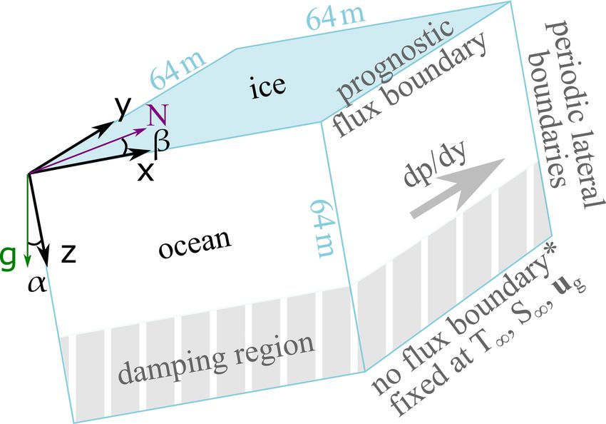
C. B. Begeman et al.: IOBL dynamics                                                                                            279

makes with north, and α is the slope angle from horizontal         2.2   Boundary conditions for ice-shelf melting
or equivalently the angle between the z axis and g. For the
rotated Coriolis vector f ,  is the rotation rate, and φ is the   Sources and sinks of momentum, as well as of heat and salt
latitude. Unless otherwise specified, quantities are oriented      due to interactions between the flow and the ice base, are
with the simulated grid.                                           parameterized as sub-grid fluxes at the top boundary. The
   The buoyancy term in Eq. (1) combines the contributions         resolved vertical fluxes at the top layer of the model go to
of the along-slope pressure gradient due to the slope of the       zero as w goes to zero according to the no-flux boundary
ice shelf in hydrostatic equilibrium and buoyancy due to           condition, and the sub-grid fluxes are determined using the
changes in density relative to the ambient density of the wa-      scheme described below in place of the AMD scheme at the
ter column ρa . We use the nonlinear equation of state from        top layer. PALM is vertically discretized such that the ice
Jackett et al. (2006) to compute densities, and ρa varies along    boundary (z = 0) is located at the edge of the top cell where
slope and with depth from the ice interface as a function of       the vertical velocity component resides, and scalar and hor-
the hydrostatic pressure:                                          izontal velocity components are located at mid-depth of the
                                                                 top cell (z = − 12 1z ). We denote the interface location with
ρa (x, y, z) = fEOS θ i (z), S i (z), p(x, y, z) ,           (7)   subscript b and the middle of the first cell below the interface
                                                                   with subscript 12 .
where the superscript i denotes the initial state. The refer-         Sub-grid momentum fluxes are parameterized according
ence density ρ0 is evaluated in the center of the x–y plane        to the law of the wall following a linear stability function for
(ρ0 (z) = ρa (xmid , ymid , z)). We neglect hydrostatic pressure   stabilizing buoyancy forcing as in Vreugdenhil and Taylor
gradients along slope except through ρa in the buoyancy            (2019):
term. For the maximum slope simulated in this study, the                              h            i
                                                                                     κ ui z 1 − ui,b
maximum hydrostatic pressure gradient is on the order of
                                                                   w 00 u00i b = u∗         2                                 (8)
100 Pa m−1 . This simplification has the advantage of avoid-

                                                                                   ln z 1 /z0 − 9m ζ 1
ing pressure discontinuities across the periodic boundary.                           2                2

   The terms on the right-hand side of the heat and salt con-      for the horizontal velocity components (i.e., i = 1, 2). ζk =
servation equations (Eqs. 3 and 4) are advection by the re-        zk /LO is the depth from the boundary scaled by the Monin–
solved flow, turbulent transport by the sub-grid-scale fluctu-     Obukhov length, u∗ is the friction velocity, and z0 is the
ations, and the source and sink terms 8θ,S . The source and        roughness length. The horizontal velocity at the boundary
sink terms are zero in our simulations because we treat heat       ui,b is always 0. The Monin–Obukhov length LO , computed
and salt fluxes due to melting at the boundaries through the       following McPhee et al. (1987), is a function of both u∗ and
sub-grid vertical flux term, as discussed in Sect. 2.2.            the melt rate. The stability function 9m is linear with the
   We employ PALM’s implementation of the Piacsek and              scaled depth.
Williams (1970) second-order advection scheme for momen-
tum and scalars and a third-order Runge–Kutta time-stepping        9m (ζ ) = 1 + βm ζ                                           (9)
scheme. We also use the Temperton (1992) fast Fourier trans-       This parameterization assumes that Coriolis forces are not
form algorithm for the pressure solver.                            locally dominant in the momentum balance.
   The turbulence closure scheme is anisotropic minimum               Similarly, the sub-grid fluxes of scalars are parameterized
dissipation (AMD; Rozema et al., 2015) employing the ex-           by
tension to scalars introduced by Abkar et al. (2016). We
validated our implementation against the stable atmospheric        w 00 θ 00 b = 0θ u∗ θ 1 − θb , w00 S 00 b = 0S u∗ S 1 − Sb , (10)
                                                                                     2                             2
boundary layer test case published in Abkar and Moin (2017)
and Stoll and Porté-Agel (2008). We follow the Abkar and           where the exchange coefficients are defined with two terms,
Moin (2017) model setup exactly and chose their moderate           one representing turbulent transfer within the turbulent sur-
resolution with 72 × 72 × 72 grid points. Our results are in       face layer and one representing molecular transfer within
good agreement with the Abkar and Moin (2017) solution             the viscous sublayer following McPhee et al. (1987) (their
employing another LES model with AMD (boundary layer               Eq. 11).
height differs by < 10 %) and other LES models with differ-
                                                                   0θ = 0θ,turb + 0θ,mol , 0S = 0S,turb + 0S,mol            (11)
ent turbulence closures (Fig. S1 in our Supplement and their
Fig. 1 and references therein). Typical sub-grid-scale mo-         The turbulent flux component follows a shape function con-
mentum and scalar diffusivities in our sub-ice-shelf simula-       sistent with the parameterization of momentum fluxes in
tions of stratified turbulence range from 10−5 to 10−4 m2 s−1      Eq. (8):
in the upper two-thirds of the domain where damping is not                        h                  i
applied (the damping methodology is discussed in Sect. 2.3).       0θ,turb = κ −1 ln z 1 /z0 − 9θ ζ 1 ,
                                                                                         2              2
                                                                                          h               i
                                                                                      −1
                                                                          0S,turb = κ      ln z 1 /z0 − 9S ζ 1 ,         (12)
                                                                                               2               2

https://doi.org/10.5194/tc-16-277-2022                                                      The Cryosphere, 16, 277–295, 2022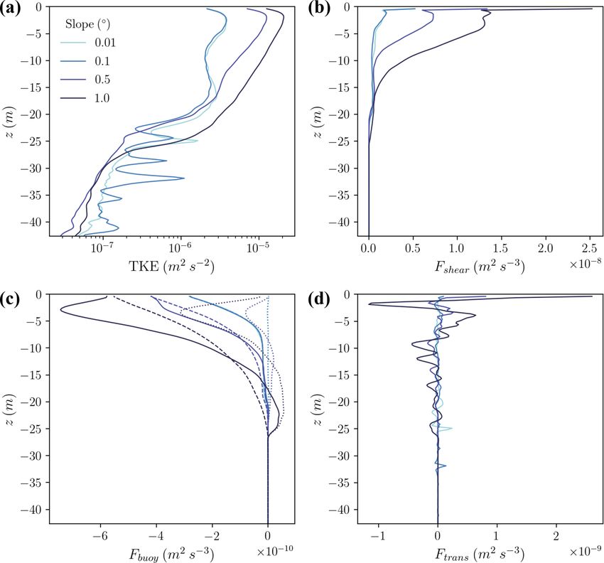
280                                                                                                 C. B. Begeman et al.: IOBL dynamics

with analogous stability functions to momentum, Eq. (9),

9θ (ζ ) = 1 + βθ ζ, 9S (ζ ) = 1 + βS ζ.                             (13)

The coefficients of these stability functions are chosen as in
Zhou et al. (2017) and are given in Table S1. The molecular
flux components are constant in our simulations following
McPhee et al. (1987) and are also given in Table S1. If a por-
tion of the ice face experiences freezing, 0θ and 0S are set to
a higher value, indicating destabilizing fluxes (0f , Table S1).
   Taking into account the role of meltwater advection,
Eq. (10) is replaced by the following “virtual” freshwater flux
form in our implementation (Asay-Davis et al., 2016; Jenkins
et al., 2001).                                                               Figure 1. Schematic of the simulated ocean domain with back-
                 "                  #                                        ground pressure gradient dp/dy. The purple arrow is oriented north,
                           Sb − S 1                                        and the green arrow is aligned with gravitational acceleration. The
                                  2
w00 θ 00 b = − u∗ 0θ − 0S              θb − θ 1             (14)             ∗ signifies that the bottom boundary condition is Dirichlet, but there
                              Sb              2
                                                                             is also no flux as a result of damping.
                 "                  #
                           Sb − S 1
  00  00                          2
w S b = − u∗ 0S − 0S                   Sb − S 1             (15)
                              Sb               2

                                                                             the mean flow, which is geostrophic in the far field where
The temperature and salinity at the ice–ocean interface, θb                  buoyancy does not modify the flow. We choose a pressure
and Sb , are unknown. Three equations are used to solve for                  of 800 dbar at the top of the domain, an intermediate choice
these quantities and the melt rate m, the so-called three-                   given that the depth of ice-shelf bottoms ranges over an order
equation parameterization.                                                   of magnitude (roughly −2000 to −200 m). The potentially
                                                                             dynamically relevant differences between conducting these
ρcp w 00 θ 00 b = −ρw mL                                            (16)
                                                                             simulations at surface pressure and 800 dbar are that the first
  ρw 00 S 00   b   = −ρw mSb                                        (17)     derivative of the freezing temperature with respect to salinity
          θb = θf (p, Sb )                                          (18)     is 20 % smaller and the first derivative of density with respect
                                                                             to salinity is about 2 times larger.
These equations specify that heat and salt are conserved                        We set von Neumann boundary conditions at the top
at the ice–ocean interface (Eqs. 16 and 17), and the inter-                  boundary corresponding to the dynamic sub-grid momentum
face temperature is fixed at the local freezing temperature θf               and scalar fluxes (Eqs. 8, 14, and 15) as resolved fluxes go
(Eq. 18). Equation (16) assumes that the conductive heat flux                to zero at a no-penetration boundary. The roughness length
into ice is negligible. ρw denotes the density of freshwater.                (z0 in Eqs. 8 and 12) is chosen such that the equivalent drag
The freezing point is calculated using the polynomial func-                  coefficient assuming quadratic drag is 0.003, an intermediate
tion from Jackett et al. (2006).                                             value for sea ice and ice-shelf bottoms, though poorly con-
   The PALM implementation applies the fluxes w00 u00i b ,                   strained (Holland and Jenkins, 1999; Holland and Feltham,
w00 θ 00 b , and w 00 S 00 b at the center of the first grid cell from the   2006; MacAyeal, 1984; Nicholls et al., 2006). Boundary con-
boundary without interpolation (i.e., w00 X 00 b = w 00 X00 1 ). It is       ditions are Dirichlet at the bottom boundary, assigned to the
                                                                    2
noted by the PALM developers that this error was found to                    far-field temperature, salinity, and geostrophic velocity. The
be small, but we have not confirmed this for the sub-ice case.               bottom third of the domain is a sponge layer (Rayleigh damp-
This error would be small if the first ∼ 10 cm were nearly                   ing) within which velocity, temperature, and salinity are re-
a constant flux layer; McPhee (1981) hypothesized that the                   laxed toward their assigned values at the bottom of the do-
sub-ice-surface layer would be nearly but not exactly a con-                 main (Klemp and Lilly, 1978; Maronga et al., 2015). The
stant flux layer.                                                            sponge layer results in negligible vertical fluxes of heat, salt,
                                                                             or momentum across the bottom boundary because scalar and
2.3   Simulation setup                                                       velocity gradients go to 0. The flow is periodic along the x
                                                                             and y dimensions.
A schematic of the simulation domain is shown in Fig. 1. A                      We present two sets of simulations which have a base case
list of parameter choices relevant to our simulations can be                 in common. The base case has low far-field thermal driving
found in Table S1. The domain is a 64 m3 cube with hori-                     of 0.15 ◦ C, a slope of 1◦ , and vigorous far-field inertial os-
zontal resolution of 0.5 m and vertical resolution of 0.25 m.                cillations of 20 cm s−1 generated by a 0.03 Pa m−1 pressure
The ice–ocean interface is located on the top boundary of                    gradient. These conditions were chosen to favor an energetic
the domain. Large-scale horizontal pressure gradients drive                  regime, for reasons discussed in Sect. 4.1. To examine the

The Cryosphere, 16, 277–295, 2022                                                                   https://doi.org/10.5194/tc-16-277-2022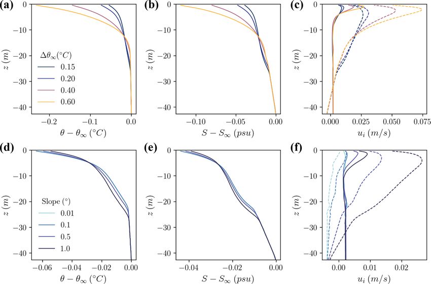
C. B. Begeman et al.: IOBL dynamics 281
relationship between thermal driving and melt rate, as well turbulent length scales and necessitates higher model resolu-
as turbulent flow characteristics, we vary the far-field ther- tion than we could computationally afford. Our simulations
mal driving from 0.15 to 0.6 ◦ C in the first set of simulations. generally show resolved turbulent fluxes exceeding sub-grid
The far-field thermal driving, 1θ∞ , is defined as the differ- turbulent fluxes by at least a factor of 2, but sub-grid tur-
ence between the far-field temperature (θ∞ ) and the freez- bulent fluxes dominate within several meters of the ice base
ing temperature based on the far-field salinity (θf (S∞ )). In where the stratification is strongest (Fig. S2). Resolved tur-
the second set of simulations, we reduce the slope from 1 bulent fluxes are also comparable to sub-grid turbulent fluxes
to 0.01◦ . The ice base always slopes to the east in the posi- late in the simulation of low-slope cases after significant TKE
tive x dimension of our domain; thus β = 90◦ . The far-field has been lost (≤ 0.1 ◦ C slopes, Fig. S2d). We evaluated the
salinity for all runs is 35 g kg−1 . Initially, both temperature effects of doubling both horizontal and vertical resolutions in
and salinity increase with depth over the upper two-thirds of a separate simulation with an otherwise identical setup to the
the domain. The background salinity stratification dominates base case, which was run for one inertial period after spin-
the density stratification, with an inverse stability ratio Rρ∗ of up. While a greater portion of the vertical heat fluxes was
20. resolved as expected, the melt rate averaged over one inertial
We initiate turbulence over the first 50 min of the simu- period only increased by 7 %, and differences in the mean
lation with perturbations to the horizontal velocity compo- state were sufficiently small to justify the use of our standard
nents on the order of 0.01 m s−1 . The simulation duration is resolution (Fig. S3).
50 h, corresponding to approximately four inertial periods of We present depth profiles of temperature, salinity, and
13 h. PALM employs adaptive time-stepping; time-steps for velocity at the end of all simulations (Fig. 3). The time-
the simulations presented here range from 0.5 to 2.75 s af- averaged far-field velocity shown in Fig. 3c and f removes
ter 2 h. By the end of our simulations, the time-mean kinetic a periodic signal from inertial oscillations of the geostrophic
energy of the flow has reached steady state. However, the tur- velocity with a characteristic magnitude of 20 cm s−1 . Ek-
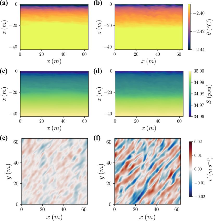
bulent intensity for all cases continues to decline, with more man rotation near the boundary can be seen in all simula-
pronounced turbulence kinetic energy (TKE) loss at lower tions (Fig. 3c, f), but for more strongly sloped runs, buoy-
slopes (Fig. 2a, d). Unless stated otherwise, the results are ancy plays an increasingly strong role in driving the mean
presented as averages over the last simulated inertial period flow near the boundary. This effect can be seen most clearly
and over the domain excluding the sponge layer. by comparing the up-slope component of the flow within
We compute an effective thermal exchange coefficient that several meters of the ice–ocean interface across the slope-
differs from that employed by the sub-grid scheme to rep- varying simulations (Fig. 3f). These mean buoyancy effects
resent the efficiency of heat exchange that may need to be increase flow velocities on the order of a few centimeters
represented to produce accurate melt rates in an ocean model per second as slope varies from 0.01 to 1◦ . Flow velocities
that does not have the vertical resolution or sophisticated near the boundary increase on the order of 10 cm s−1 as far-
turbulence closure that we employ here. This derived ther- field thermal driving increases from 0.4 to 0.6 ◦ C at 1◦ slope
mal exchange coefficient, 0T,der , can be computed using (Fig. 3c). This velocity increase is attributed to changes in
Eqs. (10) and (16) from the simulated melt rate and ocean the magnitude of buoyancy forcing near the boundary which
properties at any depth below z 1 , here chosen at −2 m. We is related to differences in melt rates. The vertical momen-
2
substitute the friction velocity computed by Eq. (8) with tum flux profiles shown in Fig. 4a and c reveal that flow is
one computed using a quadratic drag law from the veloc- accelerated (negative fluxes) over much of the IOBL, with
ity simulated 2 m below the boundary and the applied drag drag dominating only within the first few meters below the
coefficient, consistent with drag implementations in coarse- boundary.
resolution ocean models. All simulations show an evolution from the weakly strat-
ified initial conditions to more strongly stratified conditions,
particularly within the first 5 m of the ice–ocean interface
3 Results (Fig. 3b, e). In none of the simulations do we observe a well-
mixed boundary layer with respect to scalars. Rather, the
3.1 Overview of the mean simulated state simulations show varying degrees of stratification over the
first 20 m from the boundary. Stratification within the bound-
Melt rates decline over the course of the simulations (Fig. 2), ary layer increases with thermal driving (Fig. 3a, b). Thus,
preventing the identification of steady-state melt rates for the effect on stratification of the increase in melt-induced
most runs. This decline is in response to the concomitant in- buoyancy fluxes with thermal driving dominates over the
crease in stratification during the course of the simulations, increase in shear induced by the buoyant flow. Conversely,
which decreases vertical heat fluxes by reducing vertical tur- stratification decreases with increasing slope, indicating that
bulent fluctuations. We do not continue our simulations be- the increase in shear induced by the buoyant flow dominates
yond four inertial periods in the hope of reaching steady-state over the increase in melt-induced buoyancy fluxes with slope.
conditions because the increase in stratification reduces the
https://doi.org/10.5194/tc-16-277-2022 The Cryosphere, 16, 277–295, 2022
282                                                                                            C. B. Begeman et al.: IOBL dynamics

Figure 2. Time evolution of (a, d) domain-averaged, resolved turbulence kinetic energy (TKE), (b, e) melt rate, and (c, f) friction velocity
for (a–c) thermal driving simulations and (d–f) variable slope simulations. The black curve represents the same simulation in all panels in
this and subsequent figures. The analysis window, the last inertial period, is shaded.

3.2       Turbulent kinetic energy budget                               lence when ice is melting (Eq. 19). Since our simulations
                                                                        only produce melting, the vertical component is always neg-
Shear production of turbulence dominates the TKE budget.                ative (dashed lines, Fig. 5c). Over the coarse of an inertial os-
The evolution of TKE can be described by three source terms             cillation, the horizontal component of buoyancy production
and dissipation.                                                        is generally positive when the mean flow is oriented upslope
                                                                        and negative when the flow is oriented downslope. Interest-
de           du          dv g3       g1
   = −u0 w 0    − v 0 w 0 − ρ 0 w0 − ρ 0 u0                             ingly, the time-averaged effect of a slope is destruction of
dt |         dz{z        dz} ρ       ρ                                  turbulence near the boundary and production of turbulence
                             |    {z      }
                   Fshear                Fbuoy                          near the base of the boundary layer (dotted lines, Fig. 5c).
           d                                                            The net effect of both horizontal and vertical buoyancy com-
      +      (w 0 p 0 + w0 e0 ) − |{z}
                                   ε                          (19)      ponents is the destruction of turbulence throughout the IOBL
          dz
          |        {z        }   diss                                   (solid lines, Fig. 5b), with the exception of the base of the
                 Ftrans                                                 IOBL where the horizontal buoyancy component augments
                                                                        entrainment. While these complexities are intriguing from a
   Here, we characterize the evolution of resolved TKE, and
                                                                        dynamical perspective, we do not explore them further here
primes designate resolved fluctuations. Figure 5b–d show the
                                                                        since the buoyancy term is not of leading order in the TKE
source terms in this budget for the variable slope simula-
                                                                        budget.
tions; the analogous figure for the thermal driving simula-
                                                                           The transport term (Ftrans ) contains two components: ad-
tions is Fig. S4 which shows similar patterns. Shear produc-
                                                                        vection of TKE due to pressure fluctuations and turbulent ad-
tion (Fshear ) ranges from ∼ 10−9 –10−8 m2 s−3 with a maxi-
                                                                        vection of TKE. The former is negligible, reaching maximum
mum at the ice–ocean interface and local maxima in the ups-
                                                                        values on the order of 10−12 m2 s−3 , while the latter increases
lope flow within 5 m of the boundary (Fig. 5a). The increase
                                                                        turbulence at the boundary with oscillations of decreasing
in TKE throughout the boundary layer as slope increases re-
                                                                        amplitude with distance from the boundary (Fig. 5d).
flects this shear-induced turbulence (Fig. 5a).
                                                                           Dissipation (diss), the remaining term in the TKE budget,
   Buoyancy production of turbulence (Fbuoy ) is 1–2 or-
                                                                        can be inferred from the remainder of these terms and the rate
ders of magnitude smaller than shear production: ∼ 10−10 –
                                                                        of change of TKE. Since we evaluate resolved TKE (e), dis-
10−9 m2 s−3 . For a sloped ice shelf, the buoyancy term can be
                                                                        sipation here represents the transfer of energy to the sub-grid
broken into two components: the horizontal buoyancy fluxes
                                                                        scales; there is no flow of energy from sub-grid to resolved
that increase turbulence when these fluxes are oriented up-
                                                                        scales in the turbulence closure scheme. In these simulations
slope and the vertical buoyancy fluxes that decrease turbu-

The Cryosphere, 16, 277–295, 2022                                                              https://doi.org/10.5194/tc-16-277-2022
C. B. Begeman et al.: IOBL dynamics                                                                                                               283

Figure 3. Depth profiles of simulated properties as they vary with (a–c) thermal driving and (d–f) slope, averaged over the last inertial period.
(a, d) The temperature relative to far-field temperature, (b, e) salinity relative to far-field salinity, and (c, f) velocity in the y direction (solid
line, positive north, cross-slope) and in the x direction (dashed line, positive east, up-slope).

Figure 4. Vertical profiles of (a, c) momentum flux, (b, e) heat flux, and (c, f) scaled heat flux averaged over the last inertial period. The first
row shows temperature cases, and the second row shows slope cases. Momentum flux is expressed in two components: u0 w0 (dashed) and
v 0 w0 (solid). Positive flux denotes upward flux (i.e., drag). The horizontal axis limits vary between panels.

https://doi.org/10.5194/tc-16-277-2022                                                                    The Cryosphere, 16, 277–295, 2022
284                                                                                            C. B. Begeman et al.: IOBL dynamics

Figure 5. (a) Simulated turbulence kinetic energy (TKE) and (b–d) TKE source terms for variable slope simulations averaged over the
last inertial period. (b) Shear production. (c) Buoyancy production: total (solid lines), vertical component (dashed), and upslope component
(dotted). (d) TKE transport. Positive denotes production and negative destruction of TKE. Note that the x-axis scales differ between panels.

TKE is not in steady state, with an average dissipation rate            thus the velocity of the buoyancy-driven current increase.
over the course of a simulation of O(10−11 ) m2 s−3 , as seen           Since the stratification decreases with increasing slope, the
in Fig. 2a and d. Dissipation in the IOBL is on the same or-            ratio of vertical to horizontal velocity variance also increases;
der as shear production (10−9 m2 s−3 ) as all other terms in            velocity fluctuations are less confined to the slope-parallel di-
the TKE budget are small.                                               rection (Fig. S5).
                                                                           We define the base of the IOBL as the depth where the
3.3   Boundary layer turbulence                                         thermal driving relative to the far-field freezing point is 99 %
                                                                        of the far-field thermal driving. The IOBL depth increases
To demonstrate the simulated turbulent structures in this               through time, reaching 13–19 m at the end of the simula-
regime, we present horizontal and vertical cross-sectional              tions. The simulated boundary layer depth increases with the
snapshots through the domain for the two slope end-members              far-field thermal driving (from 13 to 19 m) and with ice-shelf
in Fig. 6. Turbulent structures within the IOBL are consistent          basal slope (from 15 to 19 m), reflecting the increase in flow
with propagating Holmboe shear instabilities under stable               velocities across those parameter changes which drives en-
stratification (Carpenter et al., 2010). Shear is stronger within       trainment into the IOBL. Figure 7 shows the temporal evolu-
the IOBL than at the base of the IOBL due to the concentra-             tion of IOBL depth for a few simulations, with steady IOBL
tion of buoyant plume flow near the top of the IOBL. Conse-             growth at low slopes and punctuated growth at higher slopes
quently, the amplitude of these structures increases near the           corresponding to trends in TKE.
boundary for the more strongly sloped simulations (Fig. 6).                Given the temporal variability in TKE in these simula-
The difference in IOBL turbulence with slope is perhaps best            tions, we use a threshold in dissipation rate to characterize
seen in the turbulent structures at 1 m from the ice–ocean in-          the mixing layer depth as being distinct from the mixed layer
terface (Fig. 6e, f). The structures become increasingly fila-          depth. This criterion has been deployed for stratifying ocean
mentous (i.e., near-wall streaks, e.g., del Álamo and Jiménez,          boundary layers (Franks, 2015; Sutherland et al., 2014). We
2003; Hoyas and Jiménez, 2006) and coherent as slope and

The Cryosphere, 16, 277–295, 2022                                                              https://doi.org/10.5194/tc-16-277-2022
C. B. Begeman et al.: IOBL dynamics 285 Figure 6. Instantaneous flow structures observed at 40 h in the (a, c, e) 0.01◦ slope case and (b, d, f) 1◦ slope case. (a, b) Temperature in cross section mid-way through the y axis. (c, d) Salinity in cross section mid-way through the y axis. (e, f) Resolved cross-slope velocity fluctuations at 1 m below the ice–ocean interface. Figure 7. Horizontally averaged turbulence characteristics for (a) 0.15 ◦ C thermal driving and 0.01◦ slope case and (b) 0.6 ◦ C thermal driving and 1◦ slope case. Turbulence is considered intermittent when the dissipation contour of 10−9 m2 s−3 (dashed line) reaches the boundary. Significant turbulence kinetic energy (TKE, green-yellow shading) can be present when dissipation is low. Higher TKE at −25 m at later times in (a) is due to turbulent transport, while the higher TKE at later times in (b) is due to shear production. IOBL depth is contoured in black. https://doi.org/10.5194/tc-16-277-2022 The Cryosphere, 16, 277–295, 2022
286 C. B. Begeman et al.: IOBL dynamics
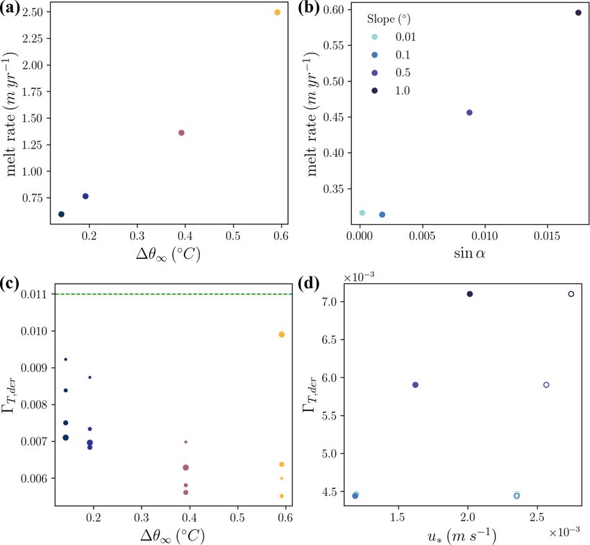
consider the mixing layer as the depth interval over which facial thermal driving as differences in friction velocity and
the horizontally and hourly averaged dissipation rate exceeds the thermal exchange coefficient are small and do not have
10−9 m2 s−3 . This mixing layer depth shows greater temporal a systematic relationship with far-field thermal driving. On
variability than the IOBL depth, as defined by scalar concen- the other hand, the derived, time-averaged thermal exchange
tration, and drops below the IOBL depth during periods of coefficient representing the efficiency of heat exchange from
enhanced entrainment (Fig. 7). −2 m depth to the ice base (0T,der ) does have a weakly nega-
There are also time periods over which the dissipation rate tive relationship with far-field thermal driving (Fig. 8c). This
drops below 10−9 m2 s−3 throughout the water column, in- indicates a decrease in the efficiency of heat exchange with
dicating intermittency in turbulence. We note that these in- increasing near-interface stratification. The highest thermal
tervals of low dissipation do not correspond to complete loss driving case shows an anomalously high thermal exchange
of TKE nor a shoaling of the IOBL depth as we have de- coefficient over the last inertial period, which features high
fined it (Fig. 7). At higher slopes (≥ 0.5◦ ), this intermittency TKE shown in Fig. 7b. We discuss these derived thermal ex-
is interrupted as inertial oscillations enhance up-slope IOBL change coefficients further in Sect. 4.2.2.
flow, increasing shear-driven mixing. This mixing front be- There is also a linear relationship between melt rate and
gins at the boundary and propagates to the base of the IOBL ice-shelf basal slope, with threshold-like behavior at slopes
over a few hours (Fig. 7b). For the less stratified, low-slope less than 0.01◦ . This linear relationship is due primarily to a
cases, the intermittency in turbulence is more frequent as the linear relationship between friction velocity and melt rate,
IOBL flows more slowly and generates less TKE production while there is a smaller (∼ 1/3 size) opposite effect from
by shear (Fig. 7a). We discuss this intermittency and its pos- decreasing interfacial thermal driving with increasing slope
sible implications further in Sect. 4.1. (not shown). These differences in friction velocity arise from
higher IOBL velocities and turbulence at higher slopes. We
3.4 Melting and its relation to thermal driving and observe threshold behavior in melting in the two lowest-
slope slope cases, which can be attributed to similar friction ve-
locities arising from similar IOBL velocities and turbulence
Average melt rates over the last inertial period range from (Figs. 8d and 3f). This behavior is discussed in more detail in
0.3 to 2.5 m (Fig. 2c, f), and average Monin–Obukhov length Sect. 4.2.1. The differences in the derived thermal exchange
scales are 3–5 m (not shown). The dominant temporal fre- coefficients with varying slopes are on the order of a 40 %
quency in melt rate is the inertial frequency, and the melt re- change as slope increases from 0.01 to 1◦ (Fig. 8d).
sponse to those oscillations is highly nonlinear. Maximum
melt rates occur when the mean flow is oriented between 3.5 Vertical structure of turbulent fluxes
the up-slope direction and the Coriolis-favored direction, and
minimum melt rates are roughly 180◦ opposed to that. These Vertical heat fluxes are shown in Fig. 4b and e. The ver-
melt rate fluctuations correspond to fluctuations in TKE tical heat flux has a maximum at the ice–ocean interface
which are reflected in the friction velocity shown in Fig. 2b and decreases throughout the IOBL, with small values be-
and e. The dominant contribution to turbulence is shear pro- low the pycnocline. Since the IOBL is fully turbulent (with
duction of TKE, which changes its distribution with depth the exception of some intermittency discussed below), the
as the mean flow profile evolves. During high-melt periods, sub-grid diffusivities of momentum, heat, and salt closely re-
the far-field flow is oriented up-slope, and shear production semble one another (Fig. S6). The vertical salt flux profiles
of TKE is concentrated near the boundary. During low-melt are shown in Fig. S7 and have a very similar shape to the
periods, the far-field flow is oriented down-slope, and shear vertical heat flux profiles.
production of TKE is concentrated a few meters away from The relatively narrow range of conditions simulated here
the boundary. Melt rate fluctuations increase in amplitude as suggests that a depth-dependent shape function for scalar
thermal driving increases and as slope increases, which we fluxes could be formulated. The distance from the interface
attribute to the increasing importance of buoyancy forcing is scaled by the Ekman depth:
in driving a near-boundary plume and thus determining the dE = (2Ke )1/2 |f3 |−1/2 , (20)
depth distribution of shear. The two simulations associated
with the highest thermal driving values, and the highest near- where Ke is the mean eddy viscosity in the turbulent bound-
boundary stratification, experience a dramatic reduction in ary layer assuming the total fluxes follow Fick’s law:
melt rates during the down-slope flow period. This coincides w 0 u0 = Ke du/dz. (21)
with reduced friction velocity (i.e., shear stress) at the ice
interface (Fig. 2b) and reduced vertical velocity fluctuations Ke profiles are shown in Fig. S8.
(not shown). The linear scaling of melt rate with thermal driving sug-
Time-averaged melt rates depend fairly linearly on far- gests a linear scaling of heat flux profiles with thermal driv-
field thermal driving (Fig. 8a, R 2 = 0.97). This is mostly at- ing. We find that this scaling largely collapses the four ther-
tributable to a linear relationship between melt rate and inter- mal driving profiles, with notable deviation from this shape
The Cryosphere, 16, 277–295, 2022 https://doi.org/10.5194/tc-16-277-2022C. B. Begeman et al.: IOBL dynamics 287
Figure 8. Melt rate sensitivity to (a) far-field thermal driving and (b) sine of the basal slope. (c) Far-field thermal driving is inversely related
to 0T,der . Dashed line denotes the value recommended by Jenkins et al. (2010). The largest points correspond to the fourth inertial cycle with
progressively smaller points for previous inertial cycles. (d) For variations in slope, the simulated friction velocity (solid points) is linearly
related to 0T,der . The inferred friction velocities used to compute 0T,der are shown with open points. Note the difference in y-axis limits
from (c). The 0.01 and 0.1◦ slope cases are overlapping.
for the run that experiences temporal gaps in shear stress dur- 4 Discussion
ing the analysis period (pink curves in Figs. 2a, 4c). The
shape of these profiles can be reasonably approximated by 4.1 Understanding IOBL turbulence and the
a linear decrease in the scaled heat flux with scaled depth limitations of a LES approach
over the boundary layer (Fig. 4c). Scalar fluxes decline near
the boundary for the 1◦ slope cases, a feature that we discuss In the simulations presented here, turbulence declines
further in Sect. 4.2.3. throughout the course of the simulation, becoming inter-
Despite melt rates scaling reasonably well with the basal mittent. The relationship between stable stratification, shear,
slope (sin α), the vertical heat flux profile does not, showing and the persistence of turbulence remains an open question
a much lower sensitivity to slope ((sin α)1/4 , Fig. 4f). There (Zonta and Soldati, 2018). Thus, it is not possible a priori
is strong agreement between the scaled vertical heat flux pro- to determine whether the level of turbulence simulated by
files at different slopes, though the threshold behavior at low this LES model is appropriate for the regime space we have
slopes noted in melt rates is replicated here. We also find sampled. While we did conduct model validation against a
that the Ekman depth is a poor predictor of boundary layer stably stratified atmospheric boundary layer test case (see
depth. This may be due to the depth-variable shear induced Sect. 2.2), the degree of stratification at the boundary in that
by buoyancy which is not reflected in the depth-mean IOBL case did not approach that simulated in the sub-ice config-
eddy viscosity used to compute the Ekman depth. We dis- uration. Fundamentally, we cannot guarantee that our LES
cuss the scaling of vertical fluxes and the possibility of their is not overly dissipative such that the TKE generated by the
parameterization in Sect. 4.2.3. resolved dynamics is lost too quickly relative to real-world
sub-ice settings.
https://doi.org/10.5194/tc-16-277-2022 The Cryosphere, 16, 277–295, 2022288 C. B. Begeman et al.: IOBL dynamics Excess dissipation could arise either through the sub-grid space for a well-mixed IOBL (Malyarenko et al., 2020). The scheme or the model numerics. We found a rapid loss of tur- observational picture is quite nuanced with a range of stratifi- bulence in PALM simulations when a dynamic Smagorinsky cation observed even within one ice shelf (Hattermann et al., turbulence closure was used, which is consistent with pre- 2012). vious studies on the limited applicability of the Smagorin- Shear-driven turbulence within the IOBL plays a central sky turbulence closure to strongly stratified flows due to the role in determining vertical heat fluxes and thus melt rates. strong anisotropy of those flows (Flores and Riley, 2011; In these simulations the destruction of TKE by the stabi- Jiménez and Cuxart, 2005). This motivated our adoption of lizing buoyancy flux is 2 orders of magnitude smaller than the AMD turbulence closure scheme (Abkar et al., 2016). shear production of TKE throughout the IOBL. Our finding However, we found that the buoyancy term added to this that shear production of TKE dominates over the buoyancy scheme by Abkar and Moin (2017) had an unrealistically term is consistent with Davis and Nicholls (2019) who found high magnitude in the vicinity of the ice base where gradi- that shear production was an order of magnitude greater than ents are large. We removed this term, as it was negligible in buoyancy destruction of TKE in the IOBL below Larsen C the simulations of Vreugdenhil and Taylor (2019) (Cather- Ice Shelf. ine Vreugdenhil, personal communication, 2020), but our un- The flux Richardson number, Rif , the ratio of buoyancy realistic solution for this term suggests that the AMD scheme flux to shear-driven TKE production, provides a measure of may not perform optimally at the resolution employed here. mixing efficiency. The simulated Rif values of 0.05–0.1 are Though the resolution of our simulations is significantly well below the critical Rif of ∼ 0.25, indicating that we are lower than that used by Vreugdenhil and Taylor (2019), it in the regime in which mixing efficiency (Rif ) decreases with enables us to extend the domain from their 2 m to 64 m to increasing stratification (Rig ) (Miles, 1961; Howard, 1961; allow for the development of a thick IOBL. Armenio and Sarkar, 2002; Peltier and Caulfield, 2003). This Strongly stratified turbulence has been associated with in- is consistent with our finding that the derived 2 m depth ther- termittent turbulence (Nieuwstadt, 2005; Wiel et al., 2012), mal exchange coefficient decreases for the high thermal driv- though there are also numerical experiments that fail to pro- ing cases which also achieve stronger IOBL stratification. duce intermittency even under strongly stable stratification Our simulations are certainly missing some sources of (Arya, 1975; Komori et al., 1983). This is not the first study TKE present in ice-shelf cavities which could modify the to find the emergence of intermittent turbulence in stably IOBL structure and mixing efficiency. These simulations did stratified, sub-ice settings (Vreugdenhil and Taylor, 2019). not include tides, which provide perturbations to the mean Donda et al. (2015) have argued that, in strongly stratified velocity that enhance melt rates and entrainment, especially flows, the cessation of turbulence is transient provided there at Filchner–Ronne (Makinson and Nicholls, 1999; Makin- are sufficiently large perturbations. This is consistent with son et al., 2011; Mueller et al., 2018). While internal gravity our finding that the temporal variability in shear over iner- waves arise in LES, in our LES model they may be of smaller tial oscillations provides sufficient perturbations to reinitiate amplitude and play a lesser role in mixing than they would in turbulence. Our simulations approach a gradient Richardson a real ice-shelf settings due to the absence of large-scale ex- number (Rig ) of 0.25, which is considered to be the approx- ternal forcings such as tides and storms, seafloor topography, imate value at which turbulence neither grows nor decays and possible resonance with the cavity geometry (Gwyther (Holt et al., 1992; Rohr et al., 1988). Thus, fluctuations in et al., 2020; Mueller et al., 2012; Padman et al., 2018; Robert- TKE are plausible at the simulated levels of stratification and son, 2013). Enhanced drag at the ice-shelf base could in- shear. However, when turbulence is intermittent, as it is in crease shear production of TKE; however, under strong strat- this study, the application of LES may be inappropriate due ification, surface roughness elements may suppress turbu- to its inherent horizontal averaging over laminar and turbu- lence rather than enhance it (Ohya, 2001). lent regions (Stoll and Porté-Agel, 2008). Thus, our results should be interpreted with caution. 4.2 Representing the IOBL and projecting ice-shelf In this study, we did not attempt to reproduce observed melt rates with ocean models conditions at a particular ice-shelf location due to the dif- ficulties of matching unobserved far-field forcings and the 4.2.1 Insights into melt rate sensitivity to ocean exclusion of tides from our simulations. Nonetheless, it ap- conditions pears as though well-mixed boundary layers are seen for a narrower range of conditions in simulations than in obser- The decline in IOBL turbulence discussed in Sect. 4.1 re- vations. The geostrophic flow chosen in these simulations is sults in declining melt rates. Thus, we could not evaluate quite strong at 20 cm s−1 , and thermal driving is relatively the relationship between melting and far-field conditions at low such that we expected to produce a well-mixed bound- steady state, which would have offered the most direct path ary layer as is observed in melting regions of the Filchner– to assessing melt rate sensitivity to ocean conditions. As dis- Ronne Ice Shelf (Nicholls et al., 2001). However, observa- cussed in Jenkins (2016), achieving steady-state solutions in tions to date are insufficient to fully characterize the regime simulations may require prescribing large-scale gradients in The Cryosphere, 16, 277–295, 2022 https://doi.org/10.5194/tc-16-277-2022
C. B. Begeman et al.: IOBL dynamics                                                                                             289

temperature. We have not included these large-scale gradi-          far-field thermal driving from these simulations is still fairly
ents in our simulations, but this may be an avenue for fu-          linear.
ture work. However, we believe that our transient solutions            The relationship between melt rate and ice-shelf basal
do provide some indications of how melt rates and boundary          slope (m ∝ (sin α)n ) combines two effects: the effect of ice-
layer properties depend on ocean temperature and ice-shelf          shelf slope on the IOBL’s mean velocity profile and the ef-
slopes. One justification for this belief is that the simulated     fect of ice-shelf slope on IOBL turbulence. In the three-
sensitivity of melt rate to ocean temperature remains consis-       equation parameterization of ice-shelf melting, the former
tently linear through all inertial periods simulated (Fig. S9).     has the strongest effect on the friction velocity as derived
On the other hand, the differently sloped simulations con-          from the mean flow velocity at a given depth, whereas the
tinue to diverge at the end of the simulation as the IOBL           latter is represented by the scalar exchange coefficients, with
accelerates (Fig. 2d–f). Nonetheless we are able to find re-        higher values indicating more efficient turbulent transport.
lationships between the vertical heat flux profiles and ocean       We return to the implications of our study for exchange co-
temperature and slope that suggest predictability of the mean       efficients in Sect. 4.2.2. As noted previously in this section,
effects of turbulence despite the transience of these simula-       while our simulations capture some of this IOBL accelera-
tions.                                                              tion, they do not reach a steady-state mean velocity profile.
   The linear relationship we find between local, far-field         Thus, we cannot fully assess the effect of ice-shelf slope on
ocean temperature and melt rates is consistent with some            the IOBL’s mean velocity profile. This effect is addressed
previous studies in ice-shelf settings (Holland et al., 2008;       by Magorrian and Wells (2016), whose scaling analysis pre-
Rignot and Jacobs, 2002; Vreugdenhil and Taylor, 2019).             dicted n = 3/2, and Little et al. (2009), who found n = 0.94
A slightly higher exponent of 4/3 is also consistent with           for the range of slopes considered here. We find that n = 1
our data (R 2 = 0.95), a value reported for the regime in           may be applicable to the shear-dominated regime, in con-
which convective instabilities control melting, while our sim-      trast to the sensitivity of n = 2/3 found in the convection-
ulations feature shear instabilities (Kerr and McConnochie,         dominated regime at higher slopes than those simulated here
2015). In contrast, in sea-ice settings this sensitivity of melt    (5–90◦ ; McConnochie and Kerr, 2018; Mondal et al., 2019).
rates to local thermal driving was found to be significantly        However, we emphasize that further investigation is needed
smaller with an exponent of 0.38 (Ramudu et al., 2018).             beyond the small number of simulations presented here to
The relationship between average ice-shelf melt rates and the       validate our results.
thermal driving for the cavity as a whole can be conceptual-           The threshold-like behavior in melt rates at very low
ized in two components. The first is the relationship between       slopes is not predicted by geostrophic balance between Cori-
the local thermal driving and melt rate, determined primarily       olis and buoyancy forcing, which dictates a linear relation-
by the local ocean turbulence. The second is the relationship       ship between sin α and IOBL velocity (Jenkins, 2016), nor
between distant thermal driving (i.e., the water masses enter-      the scaling analysis of Magorrian and Wells (2016). This
ing the ice-shelf cavity) and the strength of sub-ice-shelf cir-    threshold behavior could be produced if any additional buoy-
culation (Holland et al., 2008). Only the former is addressed       ant acceleration produced by the small increase in slope from
by this study. Our simulations do not capture the large-scale       0.01 to 0.1◦ increases both shear and dissipation, resulting
increase in overturning circulation that accompanies an in-         in a negative feedback on IOBL turbulence. This is not evi-
crease in distant thermal driving. Our simulations partially        dent in our simulations, which do not show significant differ-
capture the increase in IOBL velocity due to an increase in         ences in TKE budgets between the two runs (Fig. 5). From a
thermal driving, but the far-field velocity is unaffected. We       dynamical perspective, this may be an interesting target for
note that the often cited quadratic relationship between dis-       more highly resolved LES in the near-boundary region. How-
tant thermal driving and melt rate involves both local tur-         ever, this threshold is located at low enough slopes that it is
bulent processes and large-scale processes (Holland et al.,         likely not of significance to melt rate parameterization for
2008); studies generally find this exponent on distant thermal      coarse-resolution ocean models, so we do not devote further
driving to be between 1.5 and 2 (Favier et al., 2019; Jourdain      attention to it here.
et al., 2017; Little et al., 2009).
   To some extent, this linear relationship between far-field       4.2.2   Toward non-constant exchange coefficients in
thermal driving and melt rate is embedded in the parameteri-                melt parameterization
zation of heat fluxes employed at the ice base in these simula-
tions. Specifically, the melt rate is prescribed to have a linear   The thermal exchange coefficient as computed using Eq. (11)
dependence on the local thermal driving, based on the tem-          at 0.125 m below the ice–ocean interface (the uppermost
perature in the first model layer (Eq. 10). However, the level      grid cell) differs from that which would be implemented by
of stratification near the ice base, the buoyant acceleration of    coarse-resolution models or derived from oceanographic ob-
the IOBL plume, and the transport of heat from depth to the         servations, both of which only know ocean properties meters
IOBL all mediate the relationship between far-field thermal         to tens of meters below the ice–ocean interface. To demon-
driving and melt rates, and yet the dependence of melt rate on      strate the implications of this study for modeling endeavors,

https://doi.org/10.5194/tc-16-277-2022                                                      The Cryosphere, 16, 277–295, 2022
290                                                                                       C. B. Begeman et al.: IOBL dynamics

we computed the thermal exchange coefficient that yields the        scheme. Much greater variability in sub-grid turbulent diffu-
simulated melt rate using ocean properties (temperature and         sivities is seen over the variation in slope than the variation
velocity) 2 m below the ice–ocean interface. This depth was         in thermal driving tested here (Fig. S6).
chosen to capture the faster portions of IOBL flow, represent-         The changes in the thermal exchange coefficient with
ing a best-case scenario for high-resolution ocean models,          slope were relatively small, from 0.0045 to 0.007 between
though this depth choice is somewhat arbitrary.                     0.1 and 1◦ cases. For a coarse-resolution simulation, we an-
   These derived thermal exchange coefficients are shown in         ticipate that the failure to capture this slope sensitivity will
Fig. 8c and d. The derived thermal exchange coefficients            not be a leading source of error in melt projections. Repro-
are all less than the value of 0.011 derived from observa-          ducing an accurate friction velocity is likely of a greater con-
tions (Jenkins et al., 2010). There are two main factors that       cern. Thus, the burden of melt projection accuracy may fall
contribute to this result. The first is the choice of the pa-       more heavily on parameterizing or resolving buoyant flow
rameterization of fluxes at the ice–ocean interface (i.e., over     than on improving the slope dependence in the parameteriza-
sub-meter scales). We chose a stability-dependent parame-           tion of scalar fluxes (i.e., improving Eq. 10).
terization in which the buoyancy forcing from melting enters           These simulations do not reveal whether a similar, linear
through the Monin–Obukhov length (Eq. 9). We believe there          relationship between friction velocity and thermal exchange
is a stronger case for the flux parameterization we implement       coefficient holds when the background flow is varied rather
than for a constant thermal exchange coefficient in light of        than the slope. LES of sea-ice melting, for which there is
the success of Monin–Obukhov similarity theory (Monin and           no slope, suggests a sublinear relationship between thermal
Obukhov, 1954; McPhee, 2008), as well as the depth depen-           exchange coefficient and friction velocity (0T ∝ u∗0.5 , w0 θ 0 ∝
dence of scalar fluxes in a more highly resolved sub-ice LES        u1.5
                                                                      ∗ ; Ramudu et al., 2018). More studies are required to de-
(Vreugdenhil and Taylor, 2019). Consequently, Vreugdenhil           termine this scaling.
and Taylor (2019) also found that thermal exchange coeffi-
cients were less than the Jenkins et al. (2010) value for all       4.2.3   Toward a vertical mixing scheme for the IOBL
but the lowest thermal driving case. However, we acknowl-
edge that more validation of the sub-grid boundary flux pa-         There is reason to believe that improving ice-shelf basal melt
rameterizations is needed. The second contributing factor is        projections using ocean models will require not only an accu-
declining simulated TKE, which reduces thermal exchange             rate melt parameterization but also an improved vertical mix-
coefficients over the course of these simulations (Fig. 8c).        ing scheme. Jenkins (2021) demonstrated significantly differ-
   Our results also suggest a modest decline in the thermal         ent IOBL characteristics when KPP is the turbulence closure
exchange coefficient at higher thermal driving. This may lead       scheme in contrast to a low- or high-order scheme. The eddy
to a sub-linear relationship between thermal driving and melt       viscosity simulated by our LES model shows better agree-
rate at higher thermal driving values, though this is not ev-       ment with the viscosity solutions from Jenkins (2021) em-
ident in our simulations. The decline in exchange coeffi-           ploying the low- and high-order turbulence closure schemes
cient with thermal driving agrees with Vreugdenhil and Tay-         than that employing KPP (compare our Fig. S6 with his
lor (2019), though their sensitivity is greater than that seen      Fig. 3). Thus, this study offers additional support for the use
in this study (their Fig. 8). As shown in Fig. 8c, this rela-       of a more sophisticated turbulence closure scheme or a mod-
tionship holds during all inertial periods, with an exception       ified KPP scheme in sub-ice settings, such as one based on
during an interval of strong turbulence (see Sect. 3). Due to       the depth dependence of vertical turbulent fluxes presented
the limitations of our LES modeling discussed in Sect. 4.1,         here (Fig. 4).
we cannot recommend a best fit relationship between ther-              A complication in melt parameterization of slope effects is
mal exchange coefficient and thermal driving. Given the cli-        the differential ability of ocean models and their vertical grid
matic importance of accurately simulating high thermal driv-        configurations to capture IOBL flow. We find that this buoy-
ing regimes associated with dynamic ice-shelf thinning, LES         ant flow is concentrated in the uppermost 10 m, with peak
coupled with observational validation across thermal driving        velocities as close as 3 m from the interface. This flow is un-
regimes may be a fruitful avenue for future work.                   likely to be resolved by most ocean models, which have typ-
   We find a linear relationship between the derived thermal        ical vertical resolutions near the interface of ∼ 10 m, though
exchange coefficient and the slope of the ice-shelf base, in-       some model configurations are reaching ∼ 1 m resolutions
dicating that mixing is more efficient at higher slopes. This       (Gwyther et al., 2020). If the buoyancy-driven boundary cur-
relationship also holds for the derived friction velocity from      rent is unresolved in most coarse-resolution ocean models,
a quadratic drag law (Fig. 8d). Note that these quadratic-drag      then the friction velocity as computed from a quadratic drag
friction velocities are greater than the model’s parameteriza-      law and the velocity at the first grid cell is likely to underesti-
tion of friction velocity as the former neglects stratification     mate the true friction velocity. For instance, a simulation that
effects, while the latter includes them. This enhanced turbu-       lacks this buoyancy-induced current may look more like our
lent efficiency is due to enhanced shear instabilities and is re-   negligible (0.01◦ ) slope simulations than those with a slope
flected in turbulent diffusivities parameterized by the AMD         and may consequently underestimate melt rates. Thus, more

The Cryosphere, 16, 277–295, 2022                                                         https://doi.org/10.5194/tc-16-277-2022
You can also read