Propagating information from snow observations with CrocO ensemble data assimilation system: a 10-years case study over a snow depth observation ...
←
→
Page content transcription
If your browser does not render page correctly, please read the page content below

The Cryosphere, 16, 1281–1298, 2022
https://doi.org/10.5194/tc-16-1281-2022
© Author(s) 2022. This work is distributed under
the Creative Commons Attribution 4.0 License.

Propagating information from snow observations with CrocO
ensemble data assimilation system: a 10-years case study over
a snow depth observation network
Bertrand Cluzet1,2 , Matthieu Lafaysse1 , César Deschamps-Berger1,3 , Matthieu Vernay1 , and Marie Dumont1
1 Univ.Grenoble Alpes, Université de Toulouse, Météo-France, CNRS, CNRM, Centre d’études de la Neige, 1441 rue de la
Piscine, 38400 Saint-Martin d’Hères, France
2 WSL – Institute for Snow and Avalanche Research SLF, Davos, Switzerland
3 Centre d’Etudes Spatiales de la Biosphère, CESBIO, Univ. Toulouse, CNES/CNRS/INRA/IRD/UPS,

31401 Toulouse, France

Correspondence: Bertrand Cluzet (bertrand.cluzet@slf.ch)

Received: 20 July 2021 – Discussion started: 5 August 2021
Revised: 11 February 2022 – Accepted: 1 March 2022 – Published: 11 April 2022

Abstract. The mountainous snow cover is highly variable            Significant continuous ranked probability score (CRPS) im-
at all temporal and spatial scales. Snowpack models only           provements of about 13 % are obtained in the areas where the
imperfectly represent this variability, because of uncertain       open-loop modeling errors are the largest, e.g., the Haute-
meteorological inputs, physical parameterizations, and un-         Ariège, Andorra, and the extreme southern Alps. Over these
resolved terrain features. In situ observations of the height      areas, weather station observations are generally sparser, re-
of snow (HS), despite their limited representativeness, could      sulting in more uncertain meteorological analyses and, there-
help constrain intermediate and large-scale modeling errors        fore, snow simulations. In situ HS observations thus show
by means of data assimilation. In this work, we assimilate         an interesting complementarity with meteorological obser-
HS observations from an in situ network of 295 stations cov-       vations to better constrain snow cover simulations over large
ering the French Alps, Pyrenees, and Andorra, over the pe-         areas.
riod 2009–2019. In view of assimilating such observations
into a spatialized snow cover modeling framework, we in-
vestigate whether such observations can be used to correct
neighboring snowpack simulations. We use CrocO, an en-             1   Introduction
semble data assimilation framework of snow cover modeling,
based on a particle filter suited to the propagation of informa-   Better monitoring of the spatio-temporal variability of the
tion from observed to unobserved areas. This ensemble sys-         mountainous snow cover is paramount to improve the fore-
tem already benefits from meteorological observations, as-         casting of snow-related hazards (Morin et al., 2020) and an-
similated within SAFRAN analysis scheme. CrocO also pro-           ticipate downstream river flow (Lettenmaier et al., 2015). In
poses various localization strategies to assimilate snow ob-       mountainous terrain, the snow cover inherits a high spatial
servations. These approaches are evaluated in a leave-one-out      variability from several factors. The topography controls the
setup against the operational deterministic model and its en-      precipitation phase, air temperature, wind exposition, and ra-
semble open-loop counterpart, both running without HS as-          diation fluxes (Durand et al., 1993; Oliphant et al., 2003).
similation. Results show that an intermediate localization ra-     Wind drift redistributes snow at every scale (Mott et al.,
dius of 35–50 km yields a slightly lower root mean square er-      2018). Finally, vegetation traps the snow (Sturm et al., 2001)
ror (RMSE), and a better spread–skill than the strategy of as-     and also affects its net shortwave and longwave radiation
similating all the observations from a whole mountain range.       (Qu and Hall, 2014; Malle et al., 2019). Snowpack mod-
                                                                   els are commonly used to derive snowpack properties in the

Published by Copernicus Publications on behalf of the European Geosciences Union.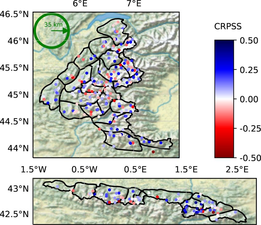
1282                                                         B. Cluzet et al.: Propagating information from snow observations

mountains. Yet, their ability to represent snow cover variabil-      the assimilation of in situ HS observations can improve sim-
ity over large areas is inherently limited by large errors in        ulations of the Météo-France operational modeling chain for
their meteorological forcings (Raleigh et al., 2015) and un-         snow cover monitoring and avalanche hazard forecasting in
certain physical parameterizations (Essery et al., 2013; Krin-       the vicinity of the measurement stations, and what is the
ner et al., 2018). In addition, explicitly accounting for pro-       most appropriate assimilation strategy for that purpose. We
cesses such as wind drift and snow–vegetation interaction            assess this in a network of in situ HS observations over the
is not yet affordable at large scales. In that context, addi-        French Alps, French Pyrenees, and Andorra, with contrasted
tional sources of information are needed to mitigate snow-           observation densities. We use CrocO, an ensemble data as-
pack modeling uncertainty in the mountains. Observations             similation system of snow cover modeling (Cluzet et al.,
from weather stations located in the mountains can be used           2021a). CrocO is built around an ensemble version of the op-
to correct Numerical Weather Prediction (NWP) model out-             erational modeling system of Météo-France (Vionnet et al.,
puts. Dedicated downscaling and analysis schemes, such as            2012; Vernay et al., 2021), accounting for modeling uncer-
SAFRAN (Durand et al., 1993) or RhiresD interpolation in             tainties from the meteorological forcings (Charrois et al.,
Switzerland (Frei and Schär, 1998), can be used to efficiently       2016; Deschamps-Berger et al., 2022) and the snowpack
reduce the large errors of the NWP models in the mountains,          model itself (Lafaysse et al., 2017; Dumont et al., 2020).
in particular by the assimilation of local precipitation obser-      CrocO includes several versions of the PF tailored for the
vations. Such approaches significantly improve snow cover            propagation of information from observed into unobserved
simulations (Durand et al., 1999; Magnusson et al., 2014).           areas (Cluzet et al., 2021a). These variants are used in a lo-
These weather stations, however, are generally located be-           calized framework, in which only observations coming from
low 1200 m (Frei and Schär, 1998; Vernay et al., 2021), and          a certain radius around the considered location are assimi-
important errors in precipitations (for example) remain at           lated (Van Leeuwen, 2009; Penny and Miyoshi, 2016; Poter-
higher elevations (Magnusson et al., 2014). Data assimila-           joy, 2016; Farchi and Bocquet, 2018). Domain localization
tion of snowpack observations may help address this issue in         is commonly used in the Ensemble Kalman Filter (EnKF;
complement to these observations. Remotely sensed retrieval          Evensen, 1994) and PF communities (Van Leeuwen, 2009;
of snow bulk properties (e.g., the height of snow (HS, m) and        Poterjoy, 2016; Penny and Miyoshi, 2016; Farchi and Boc-
the snow water equivalent (SWE, kg m−2 )) is a promising             quet, 2018). It is used to remove far-range unrealistic corre-
wealth of snowpack observations for data assimilation (e.g.,         lations in the EnKF (Houtekamer and Mitchell, 2001) and
Margulis et al., 2019) but it is inherently limited by spatio-       to circumvent the curse of dimensionality, causing the PF to
temporal gaps (De Lannoy et al., 2012), or only available at         diverge when too many observations are assimilated simul-
coarse resolutions (Andreadis and Lettenmaier, 2006). In situ        taneously (so-called PF degeneracy; Bengtsson et al., 2008).
observations of HS and SWE cover large mountainous areas             PF localization proved to be efficient in several studies (e.g.,
and are operational on a daily basis in numerous countries           Poterjoy and Anderson, 2016; Potthast et al., 2019). To as-
(e.g., Serreze et al., 1999; Jonas et al., 2009; Durand et al.,      sess the potential transfer of information, we opt for a leave-
2009b; Cantet et al., 2019). Their potential to improve local        one-out approach (e.g., Slater and Clark, 2006), whereby the
simulations is unambiguous as demonstrated by many stud-             assimilation is performed considering neighboring observa-
ies (e.g., Magnusson et al., 2017; Piazzi et al., 2018; Smyth        tions, but discarding any local observation. The assimilation
et al., 2019; Cantet et al., 2019). However, the representative-     performance can be then evaluated using these independent
ness of such observations is limited by the snow cover spa-          local observations. If such potential transfer could be demon-
tial variability (Grünewald and Lehning, 2015; Lejeune et al.,       strated, it would mean that the assimilation method is able to
2019). The potential to transfer information into neighbor-          improve simulations at a sufficient distance of available ob-
ing areas is therefore a key question when considering their         servations to be efficient over the whole simulation domain.
potential added value for snow cover modeling over large             In other words, this network of observations could be used to
domains (e.g., Slater and Clark, 2006; Liston and Hiemstra,          constrain spatialized snowpack simulations over the French
2008; Gichamo and Tarboton, 2019). This question has long            Alps, Pyrenees, and Andorra. Furthermore, the methodology
been debated. Cantet et al. (2019) successfully applied a spa-       could be applied to other areas with similar densities of ob-
tialized particle filter (PF) over a very large domain (south-       servations. To summarize, the following questions will be ad-
ern Quebec), and with a loose observation network, though            dressed in this paper:
not in a rugged terrain, i.e., less spatial variability. In alpine
terrain, Magnusson et al. (2014) and Winstral et al. (2019)            – What is the performance of data assimilation compared
showed that enhancing snow cover simulations with in situ                with the operational and ensemble models?
snow observations from a dense network in Switzerland re-
duced modeling errors over unobserved locations. It has yet            – Can data assimilation manage to propagate information
to be demonstrated that this approach can be applied over                in space?
mountainous areas with a coarser in situ observational cov-
erage (Largeron et al., 2020). Here, we investigate whether            – What is the best localization strategy for assimilation?

The Cryosphere, 16, 1281–1298, 2022                                                     https://doi.org/10.5194/tc-16-1281-2022
B. Cluzet et al.: Propagating information from snow observations 1283
– Could an increased observation density yield better re-
sults for assimilation?
The study area, observations, modeling chain, and data as-
similation scheme are described in Sect. 2. In Sect. 3, the
evaluation strategy and scores are presented. The results are
presented and discussed in Sects. 4 and 5. We finally con-
clude and open research perspectives in Sect. 6.
2 Material and methods
2.1 Study area and observations
The study area spans the French sides of the Alps and
Pyrenees and Andorra. The French Alps culminate at the
Mont-Blanc (4810 m) and are higher and about two times
larger than the French Pyrenees (culminating at Vignemale,
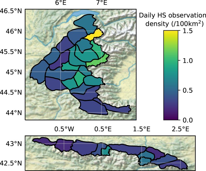
3298 m). Andorra is a principality located at the center–east Figure 1. Average daily observation density (per 100 km2 ) within
of the Pyrenees. In the following, for the sake of simplicity, each SAFRAN massif, in the French Alps (top panel) and French
we will refer to French Pyrenees and Andorra as “Pyrenees” Pyrenees/Andorra (bottom panel).
and to French Alps as “Alps”. The winter climate of the Alps
is contrasted between the north and the south. The southern
Alps are on average drier than the northern Alps (Isotta et al.,
2014). The Pyrenees are very elongated with a strong lon-
gitudinal gradient between the humid oceanic western side
to the drier Mediterranean eastern side. The elevation of the
winter snow line is around 1500 m in the Pyrenees (Durand
et al., 2012) and about 1200 m in the northern Alps (Durand
et al., 2009a). Finally, the inter-annual variability of the snow
cover is marked in both massifs (Durand et al., 2009a; Gas-
coin et al., 2015).
In this work, we perform snowpack simulations in a net-
work of 295 daily HS observations stations. A total of 217
stations are located in the Alps and 78 in the Pyrenees (of
which 7 are in Andorra). This network is an aggregate of
several data sources. Most of the observations (144 stations)
come from ski resorts, where HS is manually observed ev-
ery morning during the commercial season (mid-December Figure 2. Number of daily observations per month (a–c) and per
to April, in general). The second source is a network of cli- 300 m elevation bands (b–d) for winters 2011 (239 stations, a–b)
matological observations (77 stations) in which several me- and 2017 (250 stations, c–d) over the whole domain.
teorological parameters and HS are observed on a daily ba-
sis for the whole year. These stations are generally located
around populated areas or in ski resorts. A few sites (19 sta- sif. It is mainly explained by the variable density of ski re-
tions) come from various automated measurements in ski sorts. Although the density of observations is generally lower
resorts. Two networks of automated HS sensors were also than in the Alps, the Pyrenees exhibit two clusters of dense
used: Météo-France’s Nivôses (27 stations) and Électricité observations, in the central-western part around Bigorre and
de France (EDF) EDFNIVO stations (28 stations), the lat- in the central-eastern part close to Andorra. In the Alps, the
ter only from the winter season 2016–2017 onward. These density of observations is especially high from the northern
networks are located in remote areas and at generally higher to the south-central area. The southern massifs, as well as the
altitudes than the rest of the observations. lower altitude western massifs, generally have fewer obser-
The density of HS observations within each SAFRAN vations.
massif (Fig. 1, see Sect. 2.2.2 for more details on SAFRAN) Figure 2a–c shows the number of observations per month
is very variable, from less than 0.5 daily observations per 100 for two representative winters. It increases from 3000 during
km2 in the extreme southern Alps and western Pyrenees to fall to 6000 during January to March (when the ski resorts are
more than 10 times higher densities in the Mont-Blanc mas- open), suggesting that the beginning and end of season are
https://doi.org/10.5194/tc-16-1281-2022 The Cryosphere, 16, 1281–1298, 2022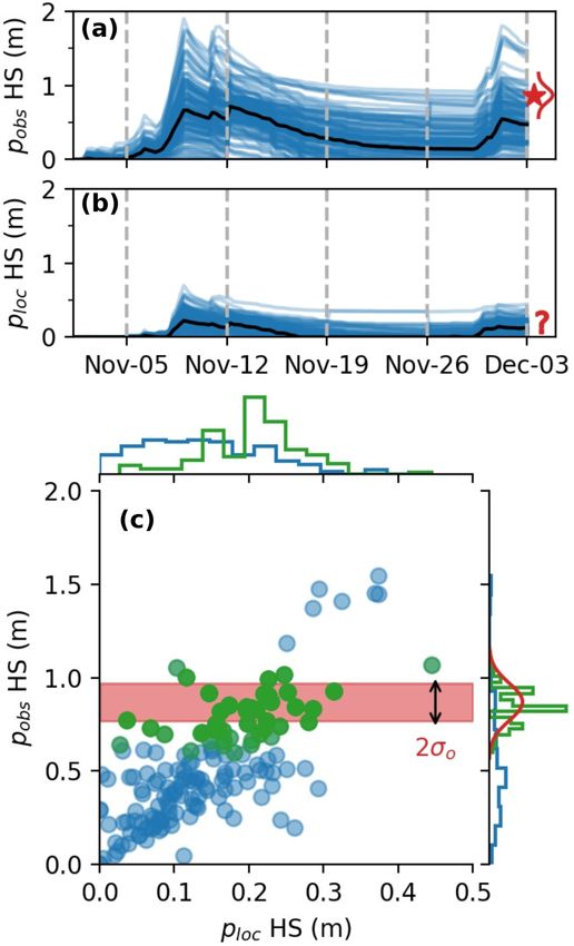
1284                                                      B. Cluzet et al.: Propagating information from snow observations

less well observed both in terms of number of observations        semi-distributed geometry, i.e within 300 m elevation bands,
and spatial coverage. Figure 2b–d shows the histograms of         aspect, and slopes, the main topographic parameters control-
the available daily observations per 300 m elevation bands for    ling the snow cover evolution. This analysis is subsequently
the same years. A notable increase in the observations count      downscaled into the specific topographic conditions (i.e., el-
above 2100 m for the 3 previous years can be explained by         evation, slope, aspect, and local topographic mask) of the
the inclusion of the EDFNIVO stations.                            simulated station (Vionnet et al., 2016). This means that a
                                                                  same analysis is applied to all the points within a same mas-
2.2     Ensemble data assimilation setup                          sif, and interpolated consistently with their topographic pa-
                                                                  rameters, while analyses for neighboring stations located in
The ensemble system consists of an ensemble of meteoro-           distinct massifs will be different.
logical forcings generated by stochastic perturbations, forc-        An ensemble of forcings was generated by applying
ing a multiphysics ensemble of snow models as described in        stochastic perturbations in the same spirit as Charrois et al.
Cluzet et al. (2020) and Cluzet et al. (2021a). The total num-    (2016) but with slight corrections in the implementation of
ber of ensemble members (also named particles in the PF           the perturbations compared with Cluzet et al. (2020, 2021a)
context) was set to 160. An open-loop run (i.e., without as-      as described in Deschamps-Berger et al. (2022). For each
similation) was performed to serve as reference. Only a few       member, perturbations are auto-correlated in time following
changes were performed in the ensemble setup, which are           an auto-regressive process and are spatially homogeneous.
described in Sect. 2.2.1 and 2.2.2.                               The perturbation parameters were taken from Charrois et al.
                                                                  (2016). Precipitation parameters were adjusted (i.e., multi-
2.2.1    Ensemble of snowpack models
                                                                  plicative noise with auto correlation time τ = 1500 h, and
The simulation setup is based on a multiphysics framework         dispersion σ = 0.5) in order to obtain a spread–skill close
representing the uncertainties of the main physical param-        to 1 for the open-loop run (see Sect. 4.1). We used these per-
eterizations of Crocus (Lafaysse et al., 2017; Cluzet et al.,     turbed analyses as input for the snowpack simulations at the
2020). However, in this paper, the advanced radiative trans-      stations.
fer scheme TARTES (Libois et al., 2013, 2015) was not
used contrary to previous studies (Cluzet et al., 2020, 2021a)    2.2.3   The particle filter in CrocO
because it requires Light Absorbing Particles (LAP) fluxes
from chemistry transport models such as MOCAGE, AL-               The PF used in this work is based on the version described
ADIN or GFDL_AR4 (Josse et al., 2004; Nabat et al., 2015;         in Cluzet et al. (2021a). Only a brief description of the pro-
Horowitz et al., 2020). To date, such products are not interpo-   cedure is given here. The ensemble is updated sequentially
lated within SAFRAN geometry and would require a specific         with the PF on each assimilation date and propagated for-
treatment and validation, going much beyond the scope of          ward until the following assimilation date. The PF is local-
this study. Instead, we opted for a single parameterization of    ized: each point receives a different analysis. Based on the
the snowpack radiative transfer, the “B60” option from Brun       comparison of neighboring simulations of HS with their cor-
et al. (1992) presented in Lafaysse et al. (2017), whereby the    responding HS observations, the PF selects a sample of the
snow albedo of a layer is a function of its age.                  best ensemble members. The idea is that if a particle is per-
                                                                  forming well against nearby observations, it should also be
2.2.2    Ensemble of meteorological forcings                      efficient locally (Farchi and Bocquet, 2018). Different lo-
                                                                  calization radii are tested in this study ranging from 17 to
Meteorological forcings are taken from SAFRAN (Système            300 km. Note that when a particle is selected by the PF, the
D’Analyse Fournissant des Renseignements Adaptés à la             full local state vector is copied: the local physical consistency
Neige; Durand et al., 1993) reanalysis over the Alps and          of the variables is preserved. Particle filter degeneracy (see
Pyrenees. SAFRAN is a surface meteorological analysis             Sect. 1) may arise even with a reduced local domain size, and
system adjusting backgrounds from NWP model ARPEGE                approaches to increase the PF tolerance may be required to
(Déqué et al., 1994) with local meteorological observations       overcome it. The localization is complemented here by two
(air temperature, pressure, precipitation, humidity) within so-   different strategies described in Cluzet et al. (2021a), infla-
called massifs of about 1000 km2 (see Fig. 1) and further         tion and k-localization, leading to the “rlocal” and “klocal”
downscaled to the stations of our study. Over the consid-         algorithms, respectively. If the initial analysis is degenerated
ered period of time, 438 observation sites provided precipita-                                                                   ∗ ),
                                                                  (i.e., the effective sample size Neff is inferior to a target Neff
tion observations to SAFRAN between November and April.           the rlocal and klocal iteratively modify the assimilation set-
These stations are mostly located at lower elevations (be-        tings to make it more tolerant, so that the PF analysis reaches
low 1500 m) as presented in Fig. 4 of Vernay et al. (2021).       a sample size of Neff  ∗ . The rlocal algorithm performs an in-

Among them, 164 of these sites correspond to locations            flation of observation errors inspired by Larue et al. (2018).
with snow depth observations included in the present study.       The klocal algorithm discards observations coming from lo-
SAFRAN analysis is issued separately for each massif in a         cations exhibiting the lower ensemble correlations with the

The Cryosphere, 16, 1281–1298, 2022                                                   https://doi.org/10.5194/tc-16-1281-2022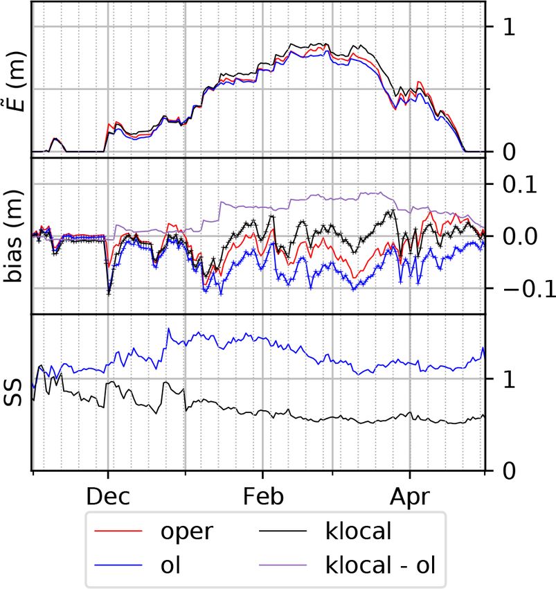
B. Cluzet et al.: Propagating information from snow observations                                                                         1285

considered location. It is important to note that inside a lo-
calization radius, the rlocal method assimilates all available
observation stations whereas the klocal method only selects
a subset of observations from locations where the ensem-
ble members are sufficiently correlated with the simulation
members of the considered point.

2.2.4   Example

This section presents an illustrative example for the propa-
gation of information with the localized PF. On 3 Decem-
ber 2009, we performed an analysis at an unobserved point
ploc (2135 m a.s.l.) using an observation from a nearby point
pobs (2293 m a.s.l., 7 km away). Figure 3a and b show the
HS simulated by the 160 ensemble members at the two lo-
cations until the considered assimilation date. The observed
HS at pobs is 0.87 m above the ensemble median at this lo-
cation (about 0.5 m). The PF will likely select the particles
that have above-average HS at pobs . Figure 3c shows the
particles’ HS values at pobs as a function of their value at
ploc . A correlation can be noted: the particles predicting the
highest HS at ploc usually also predict higher-than-average
HS at pobs . It means that the ensemble that we constructed
(see Sect. 2.2) considers that the modeling errors are linked:
if there is an underestimated snowfall in early December at
pobs , it is likely that this is also the case at ploc . The localized
PF performs an analysis for ploc by comparing the values
modeled at pobs with the available observation, thereby se-
lecting the “best” particles at pobs (c, in green). The marginal
distribution of the ensemble at pobs (right of c, in green) is
significantly sharpened compared with the background, and
is much closer to the observation. At ploc , the distribution of
the HS values of these particles is also sharper, and exhibits
higher HS than before the analysis. This example shows how
                                                                         Figure 3. Ensemble HS simulation at the observed location pobs
the localized PF has used the non-local observation at pobs to           (a) and the unobserved point where we want to perform the local
infer information about the local unobserved point ploc . This           PF, ploc (b). The median (black), assimilation dates (dashed gray
example can be generalized to the situation where multiple               lines), and the available observation on 3 December (red star, and
observations are assimilated simultaneously as done in this              probability density function, PDF, in red) are also represented. Panel
study. It also highlights the implicit importance of ensemble            (c) is a scatter plot of the ensemble members at the two locations,
correlations with distant locations: in the absence of correla-          for the background (blue) and analysis (green, superimposed on the
tion, no information can be transferred. In such a situation,            blue). Marginal distributions at the individual locations are added at
the klocal algorithm would discard the observations from the             the top and right side of the plot. The observation PDF is shown on
least areas, while the rlocal would keep them. Finally, note             the right side, with a red band showing the ±1σ range around the
that if the ensemble correlation is dramatically wrong (i.e.,            observation.
positive correlation instead of negative correlation), the anal-
ysis will degrade the ensemble performance.                              its ensemble counterpart with the assimilation switched off
                                                                         (open-loop) and the state-of-the-art operational determinis-
                                                                         tic snow cover modeling system from Météo-France (oper),
3   Evaluation strategy                                                  which consists of a default Crocus version forced by the un-
                                                                         perturbed SAFRAN meteorological forcings (Vernay et al.,
This work aims to assess the potential transfer of informa-              2021).
tion between points in an HS observation network by means
of localized data assimilation, and more specifically to ad-
dress the questions presented at the end of Sect. 1. To demon-
strate that, the data assimilation system must over-perform

https://doi.org/10.5194/tc-16-1281-2022                                                          The Cryosphere, 16, 1281–1298, 2022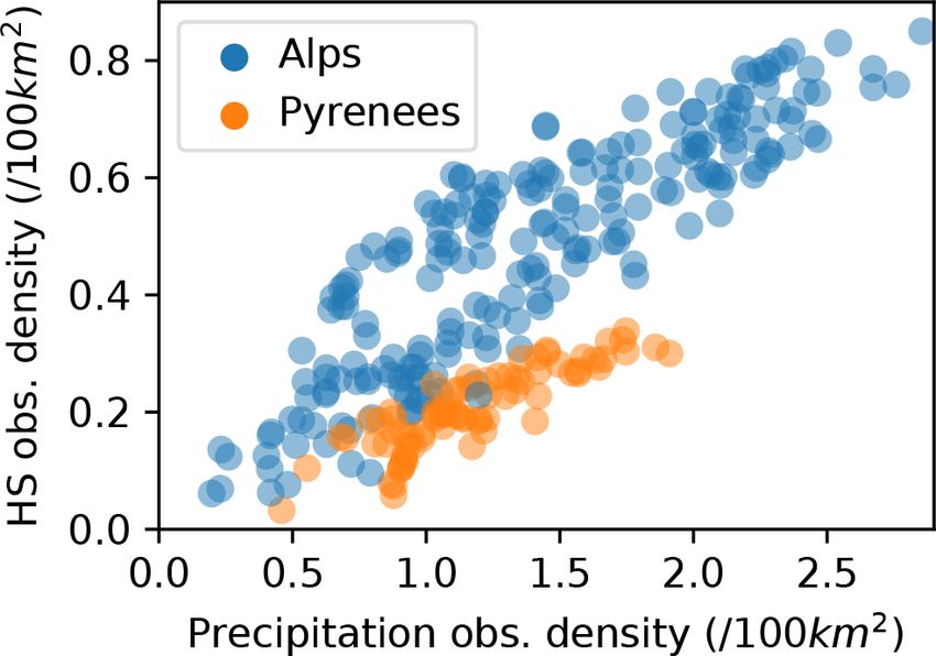
1286                                                           B. Cluzet et al.: Propagating information from snow observations

3.1    Setup                                                             The ensemble bias is defined as the average difference be-
                                                                       tween the ensemble median and the observations (Eq. 3):
Assessing the ability of data assimilation to propagate in-
formation requires use-independent data for validation. We                               Nt XN
                                                                                             pts
                                                                                1 1 X
opted for a leave-one-out setup in which local observations            bias =                    Ẽp,t − op,t .                   (3)
are removed from the set of observations used in the local PF                   Nt Npts t=1 p=1
analysis. Only weekly observations were assimilated, while
all available observations between 1 October and 30 June                 The Root Mean Squared Error of the median (RMSE) is
were kept for evaluation. There are two key design param-              computed from the AE, following (Eq. 4):
eters for the data assimilation system: the value of the local-               v
ization radius (large or small) and the choice of the PF algo-                u
                                                                              u1 1 X        Npts
                                                                                         Nt X
rithm (rlocal or klocal). Both exert a direct or indirect con-         RMSE = t                  AE2 .                            (4)
                                                                                Nt Npts t=1 p=1 p,t
trol on the number of observations simultaneously assimi-
lated by the PF, and therefore, on its potential degeneracy and
its ability to transfer information between locations. Experi-            Bias and RMSE can be computed for the oper run (treating
ments respectively combining the rlocal and klocal algorithm           it as a single-member ensemble) in order to evaluate the me-
with four different localization radii were conducted: rang-           dian performance, and can be taken over time and/or space
ing from 17 km (the radius of an idealized circular SAFRAN             by dropping the time/spatial mean in Eqs. (3) and (4). These
massif of 1000 km2 ) to 300 km (the maximal distance be-               scores are not sufficient because they reduce an ensemble to
tween two observations inside the Pyrenees and the Alps)               its median. The ensemble spread (or dispersion) σ (Eq. 5),
with two intermediate radii of 35 and 50 km. The standard              defined as the average variance, is a first metric to assess an
deviation of observation errors was set to 0.1 m as a way              ensemble reliability:
to accommodate for measurement and representativeness er-                 v
rors. Because the klocal approach does not use inflation (ex-
                                                                          u
                                                                          u1 1 1 X         Npts X
                                                                                        Nt X    Ne
cept in the case of degeneracy with only one observation),             σ= t                        (Em,p,t − E p,t )2 .           (5)
                                                                            Nt Npts Ne t=1 p=1 m=1
it is quite sensitive to the initial value of observation error.
In case of degeneracy, the smaller the observation error, the
fewer observations will be selected by the klocal algorithm.             Reliability is a desirable property for an ensemble: it
For this reason, the klocal algorithm was run with a multi-            means that all events are forecast with the right probability
plication factor of 5 on observation error variance (hence a           regardless of the probability value. The PDF of a reliable en-
fixed error standard deviation of 0.22 m), allowing more ob-           semble matches the actual PDF of observations over a large-
servations to be assimilated simultaneously.                           enough sample. We introduce the spread–skill (SS) as:
                                                                               σ
3.2    Evaluation scores                                               SS =        ,                                              (6)
                                                                              RMSE
Several metrics are used in this work to assess the perfor-
                                                                       where sigma must be computed only in the dates and loca-
mance of the oper, open-loop, and assimilation runs with re-
                                                                       tions where the RMSE is computed. For a reliable ensemble,
spect to HS observations. From the ensemble Em,p,t of Ne
                                                                       we have σ ∼ RMSE (Fortin et al., 2015), i.e., a spread–skill
members m at station p and time t, the mean can be com-
                                                                       close to unity (a necessary but not sufficient condition). This
puted using Eq. (1):
                                                                       means that the spread is on average a good estimate of the
              Ne                                                       modeling error, which is useful to make decisions. Rank di-
          1 X
E p,t =          Em,p,t .                                       (1)    agrams (Hamill, 2001) are the histogram of the position of
          Ne m=1                                                       the observation within the ensemble and enable to verify the
                                                                       reliability of an ensemble more closely (e.g., Bellier et al.,
The mean is a convenient way of synthesizing ensemble
                                                                       2017). Their flatness is a stronger condition for an ensem-
properties for evaluation; however, some artifacts can be ob-
                                                                       ble’s reliability than the SS = 1.
served with bounded variables such as HS. On a decaying
                                                                          The Continuous Ranked Probability Score (CRPS; (Eq. 7);
snow cover, for example, the mean will not reach zero un-
                                                                       Matheson and Winkler, 1976) is an aggregate, ensemble
til every member has melted. For this reason, the ensemble
                                                                       score evaluating the reliability and resolution of an ensemble
median Ẽp,t will be preferred in the following. From Ẽp,t ,
                                                                       based on a verification dataset. An ensemble has a good res-
we can compute the Absolute Error of the ensemble median
                                                                       olution when it is able to issue different forecasts on differ-
compared with the observations op,t (AE):
                                                                       ent events (contrary to the climatology; Atger, 1999). If we
AEp,t = |Ẽp,t − op,t |     ∀(p, t) ∈ [1, Npts ] × [1, Nt ],    (2)    denote Fp,t the ensemble Cumulative Distribution Function
                                                                       (CDF) and Op,t the corresponding observation CDF (Heavi-
where Nt is the number of evaluation time steps.                       side function centered on the truth value), the CRPS is com-

The Cryosphere, 16, 1281–1298, 2022                                                          https://doi.org/10.5194/tc-16-1281-2022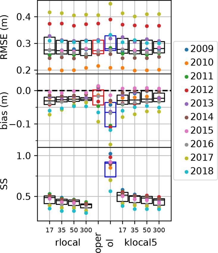
B. Cluzet et al.: Propagating information from snow observations                                                                 1287

puted at (p, t) following:
           Z
CRPSp,t = (Fp,t (x) − Op,t (x))2 dx
                R
          ∀(p, t) ∈ [1, Npts ] × [1, Nt ] .                 (7)

   The CRPS skill score (CRPSS) is commonly used to com-
pare the performance of an ensemble E to a reference R. Al-
though CRPS can be computed from a deterministic run, R
should be preferably an ensemble because comparing CRPS
of deterministic and ensemble runs mainly illustrates the ob-
vious fact that an imperfect deterministic run is a poor rep-      Figure 4. Yearly rank diagrams of the open-loop, binned into 20
resentation of a probability distribution. The following equa-     bins (i.e., for a reliable ensemble, all bars should be on the 0.05
tion is frequently used:                                           line). Values on the x axis correspond to the proportion of ensemble
                                                                   members under the observation.
                          CRPS(E)
CRPSS∗ (E, R) = 1 −               .                         (8)
                          CRPS(R)
In this formulation, if E is more skillful than R,
CRPSS∗ (E, R) will be positive, with a perfect score of 1,
while less skillful scores range between −∞ and 0, resulting
in an asymmetry between∗ positive and negative scores (i.e.,
                      CRPSS (R,E)
CRPSS∗ (E, R) = CRPSS     ∗ (R,E)−1 ). We introduce the new for-
mulation:
(
    CRPSS(E, R) = 1 − CRPS(E)
                      CRPS(R)      if CRPS(E) < CRPS(R)
                  CRPS(R)                               . (9)
    CRPSS(E, R) = CRPS(E) −1       otherwise

With such formulation, CRPS(E, R) ∈ [−1, 1] and
CRPS(E, R) = −CRPS(R, E). These properties are
important to visually compare and average improvements
(positive CRPSS) and degradations (negative CRPSS) of the
CRPS.

                                                                   Figure 5. Map of the open-loop bias (m) on each station over the
4     Results
                                                                   10 considered years (same layout as Fig. 1). SAFRAN massifs are
                                                                   outlined in black. The green circle has a radius of approximately
4.1    Performance of the reference runs
                                                                   35 km.
The operational deterministic run from Météo-France suf-
fers from significant errors (Lafaysse et al., 2013), which        in the 3 last years. In Fig. 4, yearly rank diagrams exhibit
we try to reduce by means of assimilation. The open-loop           higher frequencies in their right part, meaning that obser-
run is a first step to represent modeling uncertainty using        vations lie preferentially in the upper half of the ensemble,
an ensemble. Table 1 summarizes the yearly performance of          consistently with the negative biases exhibited in Table 1. A
both simulations over the 10 years and the 295 stations. Oper      map of the open-loop bias for each station is shown in Fig. 5.
and open-loop simulations exhibit almost identical RMSE            The bias is significantly negative in most locations, and its
scores across all years, with an average error of about 0.2–       spatial variability is high, with neighboring stations exhibit-
0.3 m. Their RMSE significantly varies (from 0.21 m in 2010        ing strong biases of opposite signs, e.g., in the central Alps.
to 0.45 m in 2017 for the open-loop) in proportion with the        Around Andorra and in the southern Alps the bias is mostly
yearly average snow depth. Oper and open-loop are slightly         negative. Some stations exhibit positive biases in the central
negatively biased, especially for the open-loop.                   Alps, but more rarely in the Pyrenees.
   Regarding ensemble metrics, the open-loop exhibits
spread–skills (SS) around 0.9–1 (SS is obtained by dividing        4.2   Overall results of the assimilation experiments
the σ column by the RMSE column in Table 1). SS ranges
from a good balance between spread and RMSE in 2009                In this work, we want to compare the performance of the
(SS = 1) to under-dispersive values (e.g., SS = 0.55 in 2018)      rlocal and klocal algorithm, with different localization radii

https://doi.org/10.5194/tc-16-1281-2022                                                   The Cryosphere, 16, 1281–1298, 2022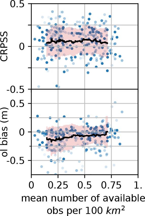
1288                                                          B. Cluzet et al.: Propagating information from snow observations

Table 1. Yearly performance of the reference runs, in terms of RMSE, bias, spread (sigma), and spread–skill (SS).

                oper mean     oper RMSE      oper bias   open-loop RMSE        open-loop sigma    open-loop bias    open-loop SS
                      (m)            (m)          (m)                (m)                    (m)             (m)
         2009         0.28           0.27       −0.02                 0.28                0.28            −0.04             1.02
         2010         0.16           0.22       −0.01                 0.21                0.18            −0.03             0.85
         2011         0.26           0.26       −0.05                 0.28                0.26            −0.10             0.92
         2012         0.44           0.37       −0.03                 0.39                0.38            −0.11             0.98
         2013         0.32           0.31        0.01                 0.32                0.29            −0.06             0.92
         2014         0.23           0.26        0.01                 0.26                0.23            −0.03             0.89
         2015         0.24           0.27        0.01                 0.27                0.25            −0.01             0.92
         2016         0.20           0.27       −0.02                 0.27                0.19            −0.07             0.70
         2017         0.41           0.41       −0.09                 0.45                0.31            −0.16             0.70
         2018         0.23           0.31       −0.07                 0.33                0.19            −0.12             0.56

(ranging from 17 to 300 km) with the oper and open-loop
runs. Figure 6 shows the yearly values of RMSE, bias, and
SS for all these runs. Results show no significant RMSE im-
provements for the assimilation runs compared with the ref-
erences. RMSE varies more from one year to another than
between assimilation configurations (algorithm and localiza-
tion radii). The median RMSE is slightly lower for the inter-
mediate localization radii of 35 and 50 km. Compared with
the open-loop, assimilation runs significantly reduce the bias
both in terms of median value, from around −0.06 to about
−0.03, and inter-annual variability. Compared with the oper
run, the absolute bias of the assimilation runs is higher on
average, but in some years, the bias is significantly reduced
(e.g., 2015, 2017, 2018).
   In terms of SS, the assimilation runs exhibit values al-
most twice as small as the open-loop run which has a me-
dian value around 0.85. The SS significantly decreases with
an increasing localization radii both for the rlocal and klo-
cal algorithm. The assimilation strategy without localization
(radii of 300 km) appears to be most efficient in reducing bi-
ases (lower absolute median, lower inter-annual variability)
but yields the lowest SS and highest RMSE of all the as-
                                                                       Figure 6. Yearly scores of RMSE (top panel), bias (middle panel),
similation runs suggesting that this approach is not the most
                                                                       and spread–skill (SS, bottom panel), for the assimilation experi-
desirable. The most selective localization strategies (radii of        ments compared with the oper and open-loop (ol) scores from Ta-
17 km) achieve the highest SS, but their inter-annual per-             ble 1. On the background are displayed the corresponding boxplots
formance variability is higher than for the other localization         and medians (black bars).
radii.

4.3    Factors of variability of the assimilation skill
                                                                       4.3.1    Spatial variability
In the following, we will investigate the different factors in-
fluencing the skill variability of the assimilation runs. As de-       Figure 7 shows boxplots of the daily deviation values (dif-
scribed in the previous Sect. 4.2, there are only small skill          ference between the model median Ẽp,t and the observation
differences between the localized radii of 17–50 km, and be-           op,t ) for the klocal and the reference runs grouped per 500 m
tween the rlocal and klocal algorithm. For the sake of illus-          elevation classes. The bias of the oper varies from slightly
tration, we decided to focus on the assimilation configuration         positive values between 1000 and 1500 m to negative val-
yielding the lowest median RMSE. This configuration, the               ues in the range 1500–2500 m to finally a positive bias at the
klocal with a 35 km localization radii, is further referred to         highest elevations. The open-loop exhibits a similar pattern,
as “klocal” configuration.                                             with a negative shift. The klocal algorithm seems to temper

The Cryosphere, 16, 1281–1298, 2022                                                         https://doi.org/10.5194/tc-16-1281-2022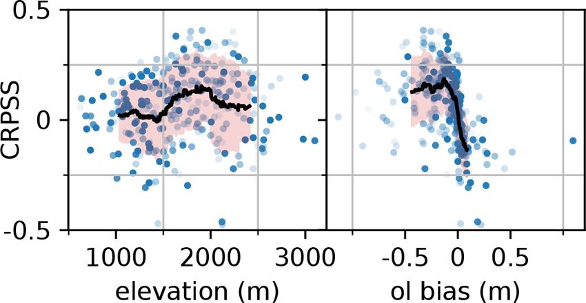
B. Cluzet et al.: Propagating information from snow observations                                                                         1289

Figure 7. Notched boxplots of the daily difference between mod-
eled and observed values (over the 10 years) of the oper (red), open-   Figure 9. Scatterplot of the CRPSS of the klocal run compared with
loop median (blue) and klocal (35km) median (black), by 500 m-          the open-loop for each station over the 10 years, as a function of the
wide elevation bands. Occurrences when the three differences are        station elevation (left panel) and the open-loop bias at each station
equal to zero are excluded.                                             (right panel). The transparency of the points is related to the propor-
                                                                        tion of available observations over the validation period. The black
                                                                        line denotes a 51-stations-wide CRPSS rolling average, with an or-
                                                                        ange shading ±1σ . This average is weighted proportionally to each
                                                                        station transparency.

                                                                        dation of skill by the analysis (negative CRPSS). The aver-
                                                                        age CRPSS varies with the altitude, increasing from a very
                                                                        low skill (0–0.03) in the range 1000–1500 m to a significant
                                                                        skill (0.1–0.15) between 1600 and 2000 m, finally decreas-
                                                                        ing to about 0.05 above 2000 m. Given the strong link be-
                                                                        tween the bias of the open-loop reference and the elevation,
                                                                        the CRPSS was also plotted against the bias of the open-loop
                                                                        in Fig. 9b. The CRPSS exhibits significant averaged positive
                                                                        values (0.13–0.2) for strong negative biases, under −0.1. The
                                                                        CRPSS varies from null performance around null bias to sig-
                                                                        nificant negative performance for positive biases (−0.12).
                                                                           The density of available observations was identified as an
                                                                        important factor for the success of the assimilation of in situ
                                                                        measurements (Winstral et al., 2019; Largeron et al., 2020).
                                                                        We define the observation density as the average number of
Figure 8. Same as Fig. 5, showing the CRPSS of the klocal against
the open-loop over the 10 years.                                        observations available on each analysis date, divided by the
                                                                        area of the localization disk. Figure 10a shows the values of
                                                                        CRPSS as a function of the observation density. CRPSS val-
                                                                        ues are rather spread, and do not seem to vary much with the
these elevation biases, with lower biases (in absolute value)           observation density. In Fig. 10 (bottom panel), the open-loop
than the oper both at higher and intermediate elevations.               bias is also plotted against the observation density, showing
   Figure 8 shows the CRPSS of the klocal (using the open-              that the highest biases are obtained for the lowest observation
loop as reference) at each station, over the 10 years. Overall          densities, although there cannot be any causal relationship as
performance is only slightly positive (blue), but with a non-           HS observations are not assimilated in the open-loop.
negligible minority of station showing negative CRPSS (red)
denoting a degradation of performance. Some “clusters” of               4.3.2   Temporal variability
good performance also appear, as in the central-eastern Pyre-
nees (Andorra and Haute Ariège) or the southern Alps, while             Time series of ensemble bias can also provide information
the performance in the central Alps and central-western Pyre-           on their nature and origin. Figure 11 shows the time series
nees seems poor.                                                        of domain-wide ensemble median Ẽ against the bias and SS
   Figure 9a represents the CRPSS as a function of the station          of the several runs in 2009. This year is representative of
elevation. On average, the analysis exhibits positive CRPSS             the different runs behaviors over the 10 years. The bias of
(between 0 and 0.15) showing that it is more skillful than              the oper run is negative except in April during the melting
the open-loop. CRPSS values exhibit a significant spread (of            season. During this year, the bias of the klocal run is cen-
about 0.2) which results in a number of stations with a degra-          tered on zero from mid-January to the end of April. The

https://doi.org/10.5194/tc-16-1281-2022                                                         The Cryosphere, 16, 1281–1298, 2022
1290 B. Cluzet et al.: Propagating information from snow observations
Figure 10. CRPSS of the klocal PF as a function of the average den- Figure 11. Time series of domain-averaged ensemble median (Ẽ)
sity of available observations (top), and open-loop bias as a function (top), bias (center), and spread–skill (SS, bottom) for the winter
of the average density of observations (per 100 km2 ; bottom). season 2009–2010, for the oper (red), open-loop (blue), and klocal
(black). The bias difference between the klocal and the oper is also
plotted in mauve in the middle panel. Dashed vertical lines corre-
spond to the assimilation dates. The onset (October) and late season
open-loop is negatively biased for the whole season. Con- (June to July) are not plotted for the sake of clarity.
sistently, the ensemble median is the highest for the klocal
run. The most interesting feature here is that the biases of all
the simulations are increasing (in absolute value) on several
drops, coinciding with increases in Ẽ during solid precipi-
tation events (e.g., early December, first week of February,
late March). The bias difference between the klocal and the
open-loop (in mauve) shows the ability of the former to re-
duce this bias. This reduction is stepwise, with the strongest
reductions occurring on analyses (dashed vertical lines) dur-
ing the accumulation period (e.g., early December, and the
two first analyses of January). Between the analyses, and dur-
ing the melting season, the time evolution of the klocal bias
follows the time evolution of the open-loop bias, and the bias
difference remains more or less constant. The SS is an esti- Figure 12. Same as Fig. 4 for the klocal.
mate of the ability of ensemble systems to assess their errors
(see Sect. 3). Here, consistently with Sect. 4.2 and Fig. 6, we
note that throughout the season, the SS of the klocal is less
the observations lie about 20 % of the time in the extremal
than 1 and significantly lower compared with the open-loop.
bins of the rank diagram (twice as much as for a reliable en-
While the SS is similar in both simulations in the early sea-
semble), and preferentially above, which is consistent with
son, klocal analyses seem to coincide with reductions of SS,
the residual negative bias of the klocal simulation.
suggesting that the ensemble spread is more reduced than
its error (RMSE) by the PF. In line with the assessment of
the reliability, Fig. 12 shows the rank diagrams of the klocal
over the 10 years. Compared with the results of the open-loop 5 Discussion
in Fig. 4, these rank diagrams exhibit a U-shape, consistent
with the significant under-dispersion of the klocal. Indeed, by In the following, we analyze the strengths and weaknesses of
summing the left and right bin frequencies, we observe that the operational and open-loop simulations and comment on
The Cryosphere, 16, 1281–1298, 2022 https://doi.org/10.5194/tc-16-1281-2022B. Cluzet et al.: Propagating information from snow observations 1291
the performance of the data assimilation algorithms in com- 5.2 The PF strategies
parison with them.
In general, one of the primary motivations of the domain
5.1 Performance of the reference simulations localization is to prevent the PF from degenerating (Farchi
and Bocquet, 2018). In our case, as evidenced by the rea-
The performance of the operational simulation has been reg- sonable performance of the rlocal with a 300 km localiza-
ularly assessed until recently (Durand et al., 2009a; Ver- tion radii (e.g., therefore simultaneously assimilating up to
nay et al., 2021). Overall, it is an accurate modeling sys- 217 observations in the Alps), domain localization is not re-
tem whose potential has been demonstrated in several recent quired against PF degeneracy thanks to the mitigations (i.e.,
climate studies and projections (e.g., López-Moreno et al., inflation or k localization) developed in Cluzet et al. (2021a).
2020; Verfaillie et al., 2018). However, it exhibits a con- Here, localization is used instead to adapt to the structures of
trasted regional performance (Fig. 13 of Vernay et al., 2021), errors in the reference run. From Fig. 5, it seems that open-
and its errors are badly known at high altitude, due to the loop bias is systematic and widespread. Then a large local-
lack of observations (Fig. 12 of Vernay et al., 2021). This ization radii, averaging a significant number of observations,
is a common issue in mountainous areas (Frei and Schär, seems a good option. However, we also see regional struc-
1998) and is detrimental for the use of the operational chain tures in this bias, probably inherited from the oper (Vernay
for all applications (avalanche hazard forecasting, hydrology, et al., 2021). They are likely due to the fact that SAFRAN
etc.). Table 1 shows that the operational version of the sys- analyses are performed at the scale of the massif. To address
tem, and its ensemble version, the open-loop, have compara- this type of error, reducing the localization radii is probably
ble RMSE. The open-loop run is reliably accounting for its a better option. Finally, the error structures can depend on
modeling uncertainties and errors, since its SS is slightly be- other parameters such as the elevation, and vary in time. In
low unity over the 10 years. This means that on average, the this situation, the klocal approach might be more adapted,
ensemble spread is almost a reliable estimate of the modeling since it adjusts the observation selection on the model back-
error. This feature could be valuable for forecasters (Buizza, ground correlation patterns. However, these background cor-
2008). relation patterns could sometimes be unrealistic and, there-
Table 1, and Figs. 6 and 11 show that the open-loop is neg- fore, misleading for the algorithm.
atively biased compared with the oper. This could be due to The klocal algorithm, by construction, selects observa-
the centered stochastic perturbations (Charrois et al., 2016; tions from locations that are correlated in the model’s point
Deschamps-Berger et al., 2022), or a bias of the ESCROC of view. However, because we apply spatially homogeneous
multiphysics model configurations (Lafaysse et al., 2017). perturbations to the meteorological forcings, strong large-
However, the oper model configuration is not expected to be scale background correlation patterns are present in the open-
perfectly centered in the open-loop, as several configurations, loop, even between the Alps and Pyrenees (not shown).
such as the parameterization of surface heat fluxes, ground These strong, potentially artificial, large-scale correlation
heat capacity, or fresh snow density, strongly influence the patterns could hamper the performance of the klocal PF, lead-
resulting modeled snow depth. Strong increases in the oper ing it to assimilate very distant observation with no actual
and open-loop biases match with precipitation events, and link with the considered location. Conversely, a completely
they are only partly compensated by the following snow set- random field of perturbations would prevent the algorithm
tling period (see Sect. 4.3.2), suggesting that it is likely that from propagating any information between locations (Mag-
error compensations take place in the oper chain, between nusson et al., 2014; Cantet et al., 2019). Using a physically
solid precipitation amounts, fresh snow density, snow com- based meteorological ensemble, such as PEARP (Descamps
paction, and ablation processes as suggested by results from et al., 2015), used in Vernay et al. (2015), or AROME-EPS
Quéno et al. (2016). Evaluation with co-located SWE and HS (Bouttier et al., 2016), or spatially correlated perturbation
data would help disentangle this situation (e.g., Smyth et al., fields (Magnusson et al., 2014), could lead to more realis-
2019). Biases of the oper and open-loop strongly depend on tic correlation fields, but this goes much beyond the scope of
the altitude (Fig. 7) in a pattern that matches the evaluation this study, as actually, domain localization prevents the klo-
from Vernay et al. (2021), though on a smaller number of cal from assimilating too distant observations.
stations and considered years. They are unambiguously neg-
ative in the range 1500–2500 m, and more variable above, 5.3 Overall performance of the assimilation compared
probably due to a higher snow cover variability, and depend- with the references
ing on the considered region. In the range 1500–2500 m, this
bias may be explained by higher wind speeds than at lower Here, we discuss the ability of the proposed assimilation ap-
elevations, causing an underestimation of solid precipitation proaches (with several localization radii) to succeed in reduc-
amounts in gauges (Kochendorfer et al., 2017), and conse- ing the modeling errors from the oper and open-loop shown
quently in SAFRAN, as evidenced by Quéno et al. (2016) in Sect. 5.1. Aggregated results from Fig. 6 show that none
during strong precipitation events. of the proposed assimilation configurations enable us to sig-
https://doi.org/10.5194/tc-16-1281-2022 The Cryosphere, 16, 1281–1298, 20221292 B. Cluzet et al.: Propagating information from snow observations
nificantly reduce overall modeling errors compared with the similation strategies (Fig. 6). In additional experiments (not
operational run. However, they overcome the significant neg- shown), the assimilation frequency was reduced to 14 d, in
ative bias of the open-loop they originate from, but at the ex- order to let the ensemble spread increase between assimila-
pense of a strongly under-dispersive spread–skill. The bias tion dates. It seems a reasonable value according to, for ex-
reduction seems more efficient and stable (i.e., less variable ample, Smyth et al. (2020) and Viallon-Galinier et al. (2020),
from year to year) with the rlocal than with the klocal, and and resulted in an increased spread, but was detrimental to
with a larger localization radii, which makes sense as the the RMSE. We did not consider increasing the target effi-
open-loop bias is widespread (e.g., Fig. 11) and both tend to- cient sample size, Neff ∗ , which was set to 100. This value
wards assimilating more observations at the same time. How- is much higher than in previous studies (Larue et al., 2018;
ever, the RMSE is slightly larger for the largest localization Cluzet et al., 2021a) and was chosen as preliminary experi-
radii, and the spread–skill is strongly reduced too. ments (not shown) with values of 25 and 50 which gave an
There are two reasons why the assimilation could not out- even lower SS. Finally, the spread of the stochastic pertur-
perform the operational run in terms of RMSE. First, its er- bations on the forcings could be increased, or statistically
ror may be of the same magnitude as the natural variability calibrated distributions of the main forcing variables (e.g.,
of point scale observations, and in that case, no added value Taillardat and Mestre, 2020) could be used.
can be extracted even from nearby observations; or similarly, Nevertheless, obtaining a perfect spread–skill may be
there are too few observations to efficiently constrain model- a challenging goal for our assimilation system. Under-
ing errors. Increasing the observation density could be an op- dispersion is a common issue in the NWP (e.g., Bellier et al.,
tion to overcome this issue. However, our results do not show 2017) and snow cover modeling communities (Lafaysse
a strong relationship between assimilation skill and density et al., 2017; Nousu et al., 2019). The spatial scale of our en-
(Fig. 10; see Sect. 5.5 later on). Another explanation could semble modeling framework cannot account for two impor-
be that there still remain systematic errors to correct, namely tant processes affecting the observations at the stations: the
biases (as suggested by Fig. 7), but it is difficult to propagate variability of the meteorological conditions inside SAFRAN
information between locations. In an idealized case, Cluzet massifs, and the snow redistribution by wind (Mott et al.,
et al. (2021a) showed that the potential to propagate informa- 2018). On the one hand, the variability of the meteorological
tion from HS observations across elevations is limited. Here, conditions inside SAFRAN massifs is limited to topographic
modeling errors are not systematic and strongly vary with parameters (including local masks) so that two distant sta-
the altitude (Fig. 7). If the ensemble does not account for this tions with the same topography will receive the exact same
specific bias structure, an observation at an elevation affected forcing (especially precipitation), and the snow redistribution
by a positive bias could never help choose the best member by wind is not represented (Vionnet et al., 2018). On the other
configuration for an elevation affected by a negative bias. hand, the spatial representativeness of observations is limited
by plot-scale variability. Data assimilation is known to partly
5.4 Difficulties faced by assimilation algorithms compensate for such scale mismatches via error compensa-
tion. Error compensations are also possible between physi-
In this part, we comment the performance of the klocal with a cal processes (Klinker and Sardeshmukh, 1992; Rodwell and
localization radii of 35 km assimilation configuration against Palmer, 2007; Wong et al., 2020). For example, an ablation
the open-loop. Although it does not outperform other config- event in one observation can be compensated in the PF by
urations significantly, the klocal seems best suited to solve selecting some members with a lower precipitation factor
the bias-elevation relation in the references and an interme- or a compaction scheme with a higher settling (Deschamps-
diate localization radii enables to adapt to local error struc- Berger et al., 2022). This compensation immediately results
tures (see Sect. 5.2). The CRPS improvement is the high- in lower errors, but implicitly, the model does a wrong as-
est for intermediate elevations coinciding with the highest sumption, which results in being overconfident, thus with a
open-loop negative bias (Fig. 9), the latter being consistent lower spread. The only way to mitigate for this overconfi-
with Cluzet et al. (2021a) who showed that the largest im- dence is to account for any relevant physical phenomenon,
provements were obtained in the presence of systematic bi- which is a desirable goal but a real challenge when it comes
ases. However, the klocal is strongly under-dispersive, con- to snowdrift by wind, local meteorology, and plot-scale vari-
trary to the open-loop which achieves an SS around 1, and ability. This goal is, to date, out of reach at the temporal and
therefore is significantly less reliable as evidenced by the U- spatial scale of this study.
shaped rank diagrams in Fig. 12. As the CRPS is a measure Despite these limitations, the assimilation shows some
of both accuracy and reliability, it seems surprising to see ability to correct weaknesses in the reference runs. The first
that the klocal is more skillful than the open-loop in terms one is the significant bias above 1500 m in the reference run
of CRPS, with average positive CRPSS around 0.06 (Fig. 9). (Fig. 7). This bias probably originates from a lack of me-
This under-dispersion is not satisfactory because it implies teorological observations in SAFRAN analysis at those alti-
that the assimilation run is too confident about its simulated tudes (see Sect. 5.1 and Fig. 4 of Vernay et al., 2021). In the
distributions. This is a general issue for all the presented as- range 1500–2000 m, the klocal has a significantly lower bias
The Cryosphere, 16, 1281–1298, 2022 https://doi.org/10.5194/tc-16-1281-2022B. Cluzet et al.: Propagating information from snow observations 1293
than the open-loop. There is a lower benefit at higher eleva-
tions, above 2000 m (Fig. 9), maybe owing to the fact that
snow cover variability is higher, in particular due to stronger
winds. There are also less observations available, and a less
clear bias at this altitude (there seems to be a transition from
a negative bias to a positive bias), reducing the odds of a suc-
cessful assimilation. Unfortunately, such elevations are key
for avalanche activity (Eckert et al., 2013; Lavigne et al.,
2015). Another good feature of the assimilation is to improve
the accuracy in areas where the references are less accurate
due to a lack of meteorological observations, namely An-
dorra and Haute-Ariège in the Pyrenees, and Ubaye, Haut
Verdon, and Mercantour in the southern Alps (Fig. 8). Both
features underline the complementarity between HS obser-
vations and the meteorological observations already assimi-
lated in SAFRAN. Figure 13. Same as Fig. 4 for the klocal.
5.5 Performance in relation to the density of
observations ments in areas where a sufficient amount of meteorological
observations are already assimilated in the snowpack mod-
The density of in situ observations has been pointed out eling chain (here, in SAFRAN). The assimilation of snow
as a critical parameter for the success of data assimilation depth observations rather gives significant improvements at
(Largeron et al., 2020). Winstral et al. (2019) managed to higher altitudes, and in areas where model errors are larger,
strongly reduce modeling errors with a high observation den- generally corresponding to areas where less meteorological
sity (about 1 observation site every 100 km2 ). Because of nat- observations are assimilated. This result could be verified in
ural variability, they considered that detection of system er- future work, in either semi-distributed or distributed frame-
rors may be more difficult with a lower density. Our study works, validated by, for example, satellite retrievals of the
case explores a wide range of observation density (Fig. 10), snow cover fraction (Magnusson et al., 2014).
from about 0.1–0.8 observations every 100 km2 (account-
ing for the availability of observations). Yet, as mentioned 5.6 Towards the assimilation in a semi-distributed
in Sects. 4.2 and 5.1, the assimilation performance relative geometry?
to the open-loop does not decrease with a lower observation
density. It may be due to the fact that the assimilation is ef- The aim of this study was to assess the potential of the
ficient only for strong open-loop negative biases (Fig. 9b), assimilation of in situ HS observations to correct nearby
which seem the highest where the station density is the low- simulations, in view of applying it in a semi-distributed or
est (Fig. 10b). In other words, the assimilation cannot outper- distributed framework (Cluzet et al., 2021a), in a strategy
form the open-loop in the most densely observed areas (e.g., similar to that of Magnusson et al. (2014) and Griessinger
in the northern Alps, where the observation density is similar et al. (2019). We used CrocO (Cluzet et al., 2021a), an en-
to that in the studies of Magnusson et al., 2014 and Winstral semble system accounting for meteorological and snowpack
et al., 2019) because the open-loop performance is already modeling uncertainties, using a PF to assimilate spatialized
high there. This behavior is explained by the fact that the HS snowpack observations. The results are mitigated: an added
observation density is correlated with the density of precipi- value is observed only when initial modeling errors are large
tation observations used by SAFRAN to analyze the meteo- (Fig. 9b), similarly to results obtained by Winstral et al.
rological forcings (see Fig. 13 and Sect. 2.2.2). Both (at the (2019). In the northern Alps, western Pyrenees, and under
exception of the Nivôse and EDF nivo stations for the HS ob- 1500 m, the added value is null on average, and seems too
servations) are actually related to human implantation in the insufficient to be of real use. Over these areas, it seems that
valleys and the presence of ski resorts. A higher weather sta- there is no room for improvement with data assimilation of
tion density for SAFRAN is likely to result in more accurate point scale HS only. There, simulation accuracy may be more
meteorological forcings, thus reducing the bias of the refer- limited by snow-related processes, such as wind drift and un-
ence runs, which finally leaves less room for improvement certain physical processes resulting in snow cover variability,
by the assimilation. than by meteorological errors. The use of spatialized satellite
This assumption may guide the strategies of definition of retrievals (Margulis et al., 2019; Cluzet et al., 2020) to better
snow cover networks, not only in terms of observation den- constrain snow cover variability, or a finer correction of me-
sity but also in terms of localization. Our study suggests teorological forcings using radar precipitation data (e.g., Bir-
that snowpack observations do not yield significant improve- man et al., 2017; Le Bastard et al., 2019) in combination with
https://doi.org/10.5194/tc-16-1281-2022 The Cryosphere, 16, 1281–1298, 2022You can also read