A Parallel Voronoi-Based Approach for Mesoscale Simulations of Cell Aggregate Electropermeabilization
←
→
Page content transcription
If your browser does not render page correctly, please read the page content below
A Parallel Voronoi-Based Approach for Mesoscale Simulations of Cell
                                                                   Aggregate Electropermeabilization

                                                                  Pouria Mistania , Arthur Guitteta , Clair Poignardc , Frederic Giboua,b
                                                          a Department
                                                                    of Mechanical Engineering, University of California, Santa Barbara, CA 93106-5070
                                                             b Department
                                                                       of Computer Science, University of California, Santa Barbara, CA 93106-5110
                                                     c Team MONC, INRIA Bordeaux-Sud-Ouest, Institut de Mathématiques de Bordeaux, CNRS UMR 5251 &

                                                               Université de Bordeaux, 351 cours de la Libération, 33405 Talence Cedex, France.
arXiv:1802.01781v1 [physics.comp-ph] 6 Feb 2018

                                                  Abstract
                                                  We introduce an approach for simulating mesoscale electropermeabilization of a cluster of cells.
                                                  We employ a forest of Octree grids along with a Voronoi mesh in a parallel environment and
                                                  in the context of the level-set method that exhibits excellent scalability. We exploit the electric
                                                  interactions between the cells through a nonlinear partial differential equation that is generalized
                                                  to account for the permeability of the cell membranes. We use the Voronoi Interface Method
                                                  (VIM) to accurately capture the sharp jump in the electric potential on the cell boundaries. The
                                                  case study simulation covers a volume of (1 mm)3 with more than 31 000 well-resolved cells with
                                                  a heterogenous mix of morphologies that are randomly distributed throughout the domain. We
                                                  follow the dynamical evolution of more than 228 000 000 nodes through timescales that enable the
                                                  unprecedented numerical studies of the electropermeabilization effects in the cluster-scale. Our
                                                  simulations qualitatively replicate the shadowing effect observed in experiments and reproduce
                                                  the time evolution of the impedance of the cell sample in agreement with the trends observed in
                                                  experiments. This approach sets the scene for performing homogenization studies for understanding
                                                  and exploiting the effect of cluster environment on the efficiency of electropermeabilization.
                                                  Keywords: Level-Set Method, Voronoi Mesh, Finite Volume Method, Quad/Oc-tree Grids,
                                                  Mathematical Biology, Electropermeabilization

                                                  1. Introduction

                                                      Electropermeabilization (also called electroporation) is a significant increase in the electrical
                                                  conductivity and permeability of the cell membrane that occurs when pulses of large amplitude (a
                                                  few hundred volts per centimeter) are applied to the cells: due to the electric field, the cell membrane
                                                  is permeabilized, and then non-permeant molecules can easily enter the cell cytoplasm by diffusion
                                                  through the electropermeabilized membrane areas. The rationale of the phenomenon lies in the
                                                  fact that since they are mainly composed of phospholipids and proteins, the cell membranes behave
                                                  like a capacitor in parallel with a resistor. The applied electric field is then dramatically enhanced
                                                  in the vicinity of the membrane, leading to a jump of the electric potential. This locally varying
                                                  transmembrane potential difference (TMP) can prevail over the cell membrane barrier where this
                                                  difference surpasses the electroporation threshold.
                                                      This phenomenon has since attracted increasing attention due to its capacity to facilitate tar-
                                                  geted drug delivery. This can be achieved by deliberately increasing the permeability of the cell
                                                  membranes with respect to non-permeant cytotoxic molecules such as bleomycin or cisplatin [? ].
                                                  DNA vaccination and gene therapy are other promising applications for electropermeabilization,
                                                  which enables non-viral gene transfection [20].
                                                      Despite extensive scrutiny of this phenomenon over the past few decades, no substantial evidence
                                                  of the elementary mechanism of electropermealization has been obtained. Nevertheless, the most

                                                    ∗ Corresponding   author: pouria@ucsb.edu

                                                  Preprint submitted to Elsevier                                                          February 7, 2018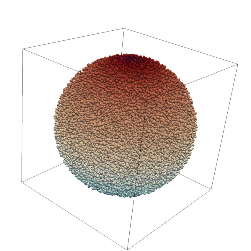
accepted theory speculates the creation of pores in the membrane as a consequence of a huge
transmembrane voltage. However these pores have not been observed yet. One important reason
behind this inefficacy is that, in the absence of cell imaging techniques in the nanometer scale,
almost all experiments to analyze this effect have used tissue scale samples to infer the underlying
molecular level processes.
Such inferences have led to the advent of different theoretical models to explain this phenomenon.
As mentioned above, membrane pore density approaches are among the most popular mechanisms.
Developments in this avenue have been carried out in the work of Debruin and Krassowska [4]
and have been augmented in [13] and [18] to incorporate the spatio-temporal evolution of the
speculated pore radii. Other attempts have been made to model the tissue scale behavior of
electropermeabilization [14].
Recently, Leguebe et al. [15] have proposed a phenomenological approach to model this effect at
single-cell scale in terms of a nonlinear partial differential equation. Their description determines
the local behaviour of each cell membrane under the influence of its surrounding electric potential
in a continuous manner. Remarkably, this representation qualifies for a multi-scale characterization
of electropermeabilization. However, we note that in practice these models embody calibrations
of free parameters that are tuned by experimenting on populations of cells and extending these
measurements to single-cell scale, oversighting multi-scale nature of electropermeabilization in the
experiments. Such approximations are inevitable in the absence of numerical tools to adjust these
models in accordance with experiments. However, recent attempts have been made in the work of
Voyer et al. [32] to theoretically extend this model to tissue scale.
We emphasize the predictability of any such model at the cell cluster regime to corroborate these
results. However, such comparisons with available experimental results were prohibitive in the case
of electropermeabilization, partially due to the enormous computational costs of such ventures as
well as the complexity of the molecular events involved in membrane electropermeabilization. To
facilitate the accurate modeling of molecular processes that regulate electropermeabilization, there
has been emerging incentive to overcome the hindering computational difficulties.
There have been recent attempts to simulate cell aggregates in tissue scale. However, these efforts
have relied on a mathematical model to mimic all the intra-cluster interactions within the cell
aggregate in terms of a semi-analytic conductivity model rather than simulating the individual
cells forming the cluster [14]. Such semi-analytic models for cluster conductivity require calibration
of free parameters that are tuned by experimenting on a sample of cells. Of course, this type of
simulations can not help to understand the molecular level processes regulating this phenomenon.
However, they serve as a means to optimize pulses used in medical treatments. We argue that such
approximations are made on the basis of simplifications in permeabilization physics that neglect
differences that arise due to, for instance, hysteresis effects in the evolution of the permeability of
the cell aggregate under different pulse scenarios and geometric configurations.
In the wake of the aforementioned arguments, the advent of “direct” tissue scale simulations seems
necessary. Such simulations not only commission better understanding of the involved molecular
processes, but also will aid developing semi-analytic models of the overall permeabilization of the
tissue under different circumstances. Such endeavors require a complete characterization of the
relevant physical parameters from cell scale physics to cluster scale configurations.
Quite recently, significant progress has been made in this venue by Guittet et al. [10]. They
have proposed a novel Voronoi Interface Method (VIM) to capture the irregular cell interface and
accurately impose the sharp TMP jump. The VIM utilizes a Voronoi mesh to capture the irregular
interface before applying the dimension-by-dimension Ghost Fluid Method [5, 12, 19]. This is aimed
to direct the fluxes normal to the interface where there is a discontinuity. This reframing the mesh
around the interface guarantees the convergence of the solution’s gradients. Also, only the right
hand side is affected by the TMP jump which simplifies the computational treatment.
In their work, Guittet et al. [10] have derived a finite volume discretization for this phenomenon and
implemented it in a serial framework. Their numerical results are in agreement with experimental
expectations. However, the computational costs of solving the involved discretization prohibited
the consideration of tissue scale simulations.
Here, we build on the method proposed by Guittet et al. [10] and generalize their approach to a

                                                  2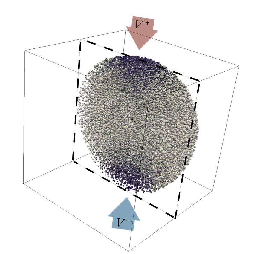
parallel environment. This parallelization empowers simulations of the single-cell model of Leguèbe
and Poignard et al. [15] at the tissue scale, hence providing a framework to validate or improve the
understanding of cell electroporation.
The structure of this paper is as follows. We introduce the mathematical model for our simulations
in section 2 and the computational strategy that we develop in section 3. We implement our
strategy in this section and present the computational performance of our implementation as well
as some preliminary demonstrations of the numerical results in sections 4. In section 5 we illustrate
the emergence of macro-level properties in the cell aggregate. We conclude with a summary of our
main results in section 6.

2. Cell membrane model

2.1. Geometric representation
    The whole simulation domain Ω is composed of the cell cytoplasm Oc and the extracellular
matrix Oe that are separated by a thin and resistive membrane denoted by Γ: [15]

                                              Ω = Oe ∪ Γ ∪ Oc                                              (1)

Figure 1 illustrates the geometry of the problem. We denote the conductivities of the materials by
σ c and σ e for the cell and the extracellular matrix respectively.

Figure 1: Illustration of a single cell immersed in the extracellular matrix. n̂ denotes the unit vector normal
to the membrane. σ is the conductivity of the materials.

2.2. Electrical model
    For simulations of electropermeabilization we solve the following boundary value problem defined
in equations (2a)–(2e). The electric potential field u in the computational domain is governed by
the Laplace equation:

                                ∆u = 0, ~x ∈ (Ωc ∪ Ωe ),                                                  (2a)

with the appropriate boundary conditions:

                                [σ∂n u]Γ = 0, ~x ∈ Γ,                                                     (2b)
                                Cm ∂t [u]Γ + S(t, [u]) [u] = σ∂n u|Γ , ~x ∈ Γ,                            (2c)
                                u(t, ~x) = g(t, ~x), ~x ∈ ∂Ω,                                             (2d)

and the homogeneous initial condition:

                                u(0, ~x) = 0, ~x ∈ Ω,                                                     (2e)

   where we used the [·] notation for the jump in the quantities:

                                            [O] = O|Γ+ − O|Γ− .

                                                        3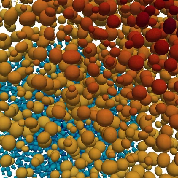
Equation 2b imposes the continuity of the electric flux across the membrane and 2c captures the
capacitor and resistor effect of the membrane. 2d is the external voltage applied on the boundaries
of the domain. In these equations, Cm and S are the capacitance and conductance of the membrane
material respectively. g(t, ~x) is the source term corresponding to the applied voltage. The effect of
electroporation current is modeled by the S(t, [u]) [u] term in equation 2c. We adopt a nonlinear
description of the conducting membrane in the next subsection. [15]
2.3. Membrane electropermeabilization model
The long-term permeabilization of the membrane is modeled by formulating the surface mem-
brane conductivity. Leguèbe, Poignard et al. modeled the surface conductivity of the membrane as
follows: [15]
Sm (t, s) = S0 + Sep (t, s) = S0 + X1 (t, s) × S1 + X2 (t, s) × S2 , ∀t > 0, s ∈ Γ (3)
In this equation S0 , S1 and S2 are the surface conductance of the membrane in the resting,
porated and permeabilized states resepectively. The level of poration and permeabilization of the
membrane are captured in the functions X1 and X2 . These are computed as a function of the
transmembrane potential difference and are valued in the range [0, 1] by definition. The ordinary
differential equations determining X1 and X2 read:
∂X1 (t, s) β0 (s) − X1
= , X1 (t, s) = 0, (4a)
∂t τep
∂X2 (t, X1 ) β1 (X1 ) − X2 β1 (X1 ) − X2
= max , , X2 (t, s) = 0. (4b)
∂t τperm τres
The parameters τep , τperm and τres are the time scales for poration, permeabilization and resealing
respectively. Furthermore, in the above equations β0 and β1 are regularized step-functions defined
as:
2
Vep
β0 (s) = e− s2 , ∀s ∈ R, (5a)
X2
− Xep
β1 (X) = e 2
, ∀X ∈ R, (5b)
where Vep and Xep are the membrane voltage and the poration thresholds respectively.
3. Computational strategy
3.1. Level-set representation
As presented by Guittet et al. [10], we describe the cells in our simulations using the level-set
method as first introduced by [27] (see [8] for a recent review) and in particular the technology on
Octree Cartesian grid by Min and Gibou [24]. To this end, we construct a spatial signed-distance
function φ relative to the irregular interface Γ such that:
d(~x, Γ) > 0, ~x ∈ Oe
φ(~x) = d(~x, Γ) = 0, ~x ∈ Γ , ~x ∈ R3 (6)
−d(~x, Γ) < 0, ~x ∈ Oc
where d(~x, Γ) is the minimum Euclidean distance from a given point in the domain to the 0-th
level-set hyperspace:
d(~x, Γ) = inf d(~x, ~y ),
y∈Γ
Figures 2(a) and 2(b) demonstrate an example of such interface representation and a sample
level-set function respectively.
4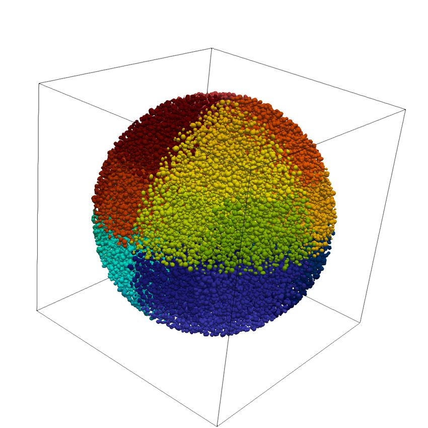
Figure 2: (left panel) The level-set representation of a single cell on an adaptive Cartesian grid at levels
(3, 8). (right panel) The membrane is resolved at the highest level while farther regions are at lower levels
representing coarser grids. Also, the level-set function φ is negative inside the cell (cooler colors) and
positive outside the cell (warmer colors).

3.2. Octree data structure and refinement criterion
    In this work we intend to simulate a large number of cells. To efficiently solve the linear system
obtained from discretizing the equations, we need to minimize the total number of nodes repre-
senting the whole domain without loss of accuracy. As the physical variations in the solution
emphatically occur close to the membrane, one needs less nodes to capture the physics at farther
regions compared to the vicinity of the cells. Hence, we utilize the adaptive Cartesian grid based
on Quad-/Oc-trees [6, 21]. A “Quad-/Oc-tree” is a recursive tree data structure where each node
is either a leaf node or is parent to 4/8 children nodes. The Octree is constructed by setting the
root of the Octree to the entire computational domain. Then higher resolutions are achieved by
recursively dividing each cell into 8 subcells (or 4 subcells in the case of Quadtrees). We use the
following refinement criteria introduced by [31] and extended by [22] to orchestrate this partitioning
of space:

   Refinement/coarsening criterion: Split a cell (C) if the following inequality applies (other-
wise merge it to its parent cell):

                                    min         |φ(v)| ≤ Lip(φ) · diag-size(C),                          (7)
                                v∈vertices(C)

where we choose a Lipschitz constant of Lip(φ) ≈ 1.2 for the level-set φ. Furthermore, diag-size(C)
stands for the length of the diagonal of C and v refers to its vertex. Intuitively, the use of the signed-
distance function in equation 7 translates into a refinement based on distance from the interface.
This process is depicted in figure 3(a). An Octree is then characterized by its minimum/maximum
levels of refinement. Figure 3(b) illustrates an example of a levels (3,8) tree meaning the minimum
and maximum number of cells in each dimension are 23 = 8 and 28 = 256 respectively.

                                                        5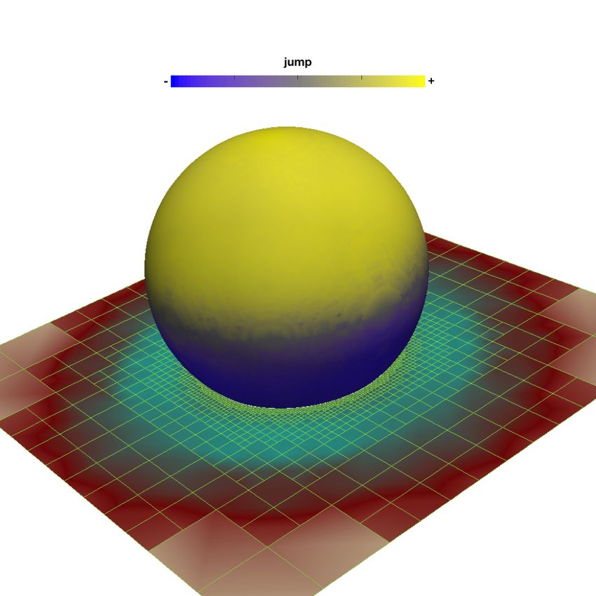
Figure 3: Illustration of an Octree mesh and its data structure. (left) Two levels of refinement are illus-
trated. (right) A portrait of 8 levels of refinement in practice. Note that each dimension is divided into at
most 28 = 256 cells.

3.3. Parallel framework
    In this work we utilize the parallelism scheme introduced by Mirzadeh et al. [25]. This scheme
is built upon the p4est software library [3]. p4est is a suite of scalable algorithms for parallel
adaptive mesh refinement/coarsening (AMR) and partitioning of the computational domain to a
forest of connected Quad-/Oc-trees. The partitioning strategy used in p4est is illustrated in figure
4. This process is briefly [3]:

   • A uniform macromesh is created;
   • A forest of Octrees is recursively constructed using all processes;
   • The produced tree is partitioned among all processes using a Z-ordering; i.e., a contiguous
     traversal of all the leaves covering all the octrees.

    The Z-ordering is then stored in a one dimensional array and is equally divided between the
processes. This contiguous partitioning optimizes the communication overhead compared to the
computation costs when solving equations in parallel. To perform the discretizations derived for
this problem, we need to construct the local Octrees from the one dimensional array of leaves.
To this end, following the method suggested by Mirzadeh et al. [25], we construct a local tree on
each process such that the levels of its leaves matches that of the leaves produced by the p4est
refinement. Each process stores only its local grid plus a surrounding layer of points from other
processes, i.e., ghost layer.

Figure 4: A “forest” composed of two Quadtrees T0 and T1 (left) partitioning the whole geometric domain
following a Z-ordering of all the octants in the domain (center). The partitioning is performed such that
each process receives equal (±1) number of contiguous octants traversing the leaves from left to right (right).
Here there are four different processes depicted by four different colors.

                                                      6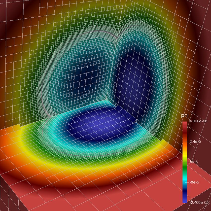
3.4. Quasi-random cell distribution
    To computationally capture the effects of a large cluster of cells under the influence of an external
electric stimulant, first we need to efficiently mimic the randomness in the distribution of the cells
while simultaneously constraining the minimum distance among the cells. For the purposes of this
work we need to simulate tens to hundreds of thousands of cells in a relatively small computational
domain to observe the relevant aspects of electropermeabilization at the tissue scale.

    In this work, we distribute the cells using the quasi-random numbers generated by the Halton
Quasi Monte Carlo (HQMC) sequence [17, 11, 2, 28]. Quasi-random sequences are more uniformly
distributed than the well-known pseudo-random sequences as illustrated in figure 5. As seen in this
figure, while uniform pseudo-random numbers suffer from local clustering and voids, the HQMC
sequence spans the space more uniformly. Mathematically, the uniformity of a sequence is measured
by its “discrepancy” which is measured by comparing the number of points in a given region of space
with the number of points expected from an ideal uniform distribution [17]. The quasi-random se-
quences are also called low discrepancy sequences as they exhibit a more uniform spatial coverage.
Remarkably, the low discrepancy characteristic is inherently built in the HQMC algorithm while
it requires further processing to enforce such a uniformity using a pseudo-random number generator.

    In this approach, we locate each cell at the next element in a three dimensional HQMC sequence
while skipping the elements that violate the minimum distance criterion to the previously located
cells. In contrast to a pseudo-random based technique, such rejections are very rare due to the
intrinsic low discrepancy of the HQMC sequence, and hence the efficiency of our technique.

   As the number of cells increases in our simulations, it becomes computationally prohibitive
to generate such a non-overlapping pseudo-random distribution of cells at high densities. Our
experiments with HQMC demonstrate that a moderately dense non-overlapping cluster of cells can
be generated at least hundreds of times faster than a pseudo-random number based technique.
Notably, initializing higher cluster volume fractions (a volume fraction of n = volume of the cells
                                                                                volume of the box ≈
O(10−1 ) ) seems completely impossible using pseudo-random number generators.

Figure 5: (left) Quasi-random number distribution versus (right) pseudo-random number distribution. The
quasi-random sequence immediately exhibits a much more uniform distribution of points.

                                                   7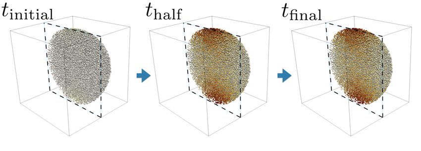
3.5. Discretization of the equations - the Voronoi Interface Method
    Here we discuss the discretization of the electropermeabilization equations introduced in section
2.2. These equations introduce non-trivial discontinuities across the interfaces of the cells. The main
difficulty arises due to boundary condition 2c which describes the jump in the potential across the
membrane. Unfortunately, this equation is an ordinary differential equation coupled to the solution
of the electric potential field, i.e., equation 2a.
    Guittet et al. [9] proposed the Voronoi Interface Method (VIM) to solve the elliptic problems with
discontinuities on irregular interfaces. Their proposed method exhibits second order accuracy by
solving the problem on a Voronoi mesh instead of the given Cartesian grid. Also, Guittet et al. [10]
extended the VIM to the case of the electropermeabilization problem including the aforementioned
non-trivial boundary condition in the discretization. In this work, we implement their modified
approach in parallel. In this section we briefly highlight this technique.
    The solver presented by Guittet et al. [9] is based on buiding a Voronoi mesh using the freely
available library Voro++ [30]. The Poisson equation is then solved on a Voronoi mesh that coincides
with the irregular interface. This introduces more degrees of freedom close to the interface and on
either side that are equidistant to the interface by design. For more details on generating the Voronoi
mesh we refer the interested reader to [9]. Here, we present the numerical scheme of Guittet et al.
[10] for completeness.
    Figure 6 illustrates the nomenclature used to describe the Vornonoi Interface Method based
discretization of this problem near the interface. First we discretize the boundary condition 2c
using a standard Backward Euler scheme:
                                                n+1             n
                                    − [u]    [u]   n+1
                                      Cm  + S n [u]    = (σ∂n un+1 )Γ ,                                    (8)
                                   ∆t
which can be rearranged to get the membrane voltage jump:
                                                                     n
                                                    n+1        Cm [u] + ∆t(σ∂n un+1 )Γ
                                              [u]          =                           ,                   (9)
                                                                     Cm + ∆tS n
In the second step we discretize the no electric flux boundary condition 2b:
                                                           uep − uei      ucj − ucp
                                                      σe             = σc           ,                    (10)
                                                              d/2            d/2
                                                          n+1
Replacing ucp by its definition uep − [u] in the above expression, coupling it with equation 9 and
rearranging the terms the final expression of uep reads:
                                               n
                                     σ c Cm [u]        σ c σ e ∆t                        σ c σ e ∆t

  uep =       σ e uei + σ c ucj +                +                 ue
                                                                       /  σ c
                                                                              + σ e
                                                                                    +                   , (11)
                                    Cm + ∆tS n     (Cm + ∆tS n )d/2 i                 Cm + ∆tS n )d/2

This equation for uep is then included in the discretization of the Laplace equation on the Voronoi
cells. Finally, we get the following expression for the potential around the interface:
                                                                                              n
                          X                  uek − uei       uj − ui                    Cm [u]
                                    sk σ e             + sσ̂         = sign(φi )sσ̂                  ,   (12)
                                                dk             d/2                  (Cm + ∆tS n )d/2
                       k∈{∂C\Γ}

where
                                                                      σc σe
                                                    σ̂ =                    e σ c ∆t      ,              (13)
                                                           σ e + σ c + (Cmσ+∆tS    n )d/2

and sign is the signum function. This is a positive definite linear system as all coefficients are
positive and the jump appears only on the right hand side of this system. We emphasize that the
points far from the interface are discretized according to the classic finite volume discretization on
the Voronoi grid. Integrations are performed with the geometric approach of Min and Gibou [23].

                                                                         8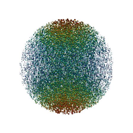
(a)                                                 (b)

                          (c)                                              (d)

Figure 6: (a) Configuration used to construct the Voronoi mesh. up corresponds to the normal projection
of nodes i and j on the interface (Γ). This point is equidistant to nodes i and j. s is the common length
(or area in 3D) of the interface between cells i and j. d is the distance between i and j. (b) The Voronoi
mesh constructed in 2D to resolve the cell interface. (c) and (d) 3D representation of the voronoi mesh in
the case of a single cell.

4. Numerical Results

    In this section we present numerical results of our implementation. Our approach is capable of
capturing the physical aspects of the interaction between the cell membrane and the applied electric
field. This is demonstrated in figure 7. As observed in this figure, the lines of the electric field are
distorted in the presence of a single cell. This provides a feedback channel for the cells to interact
over long distances and leads to environmental dependence of electropermeabilization within the
cluster environment.
    To demonstrate this effect and to showcase the computational capabilities of our approach, we
consider the case of a spherical cluster of cells confined in the center of a computational box of size
1mm on each side. Here the volume fraction of cells is set to n = 0.053 corresponding to 31, 320 cells.
This number is dictated by the minimum distance of 3×R0 between each pair of cells where R0 is the
average radius of a cell. For the purposes of the current paper, we only intend to randomly distribute
the cells with varying eccentricities. Therefore, this minimum threshold was adopted conservatively

                                                    9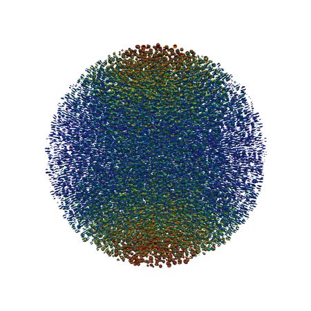
to avoid overlap between cells. A denser configuration requires a deterministic distribution to
account for the orientation of each neighboring cell to be able to fill the free space more compactly.
We leave more explicit considerations of the initial cell distribution to future work.

Figure 7: Illustration of a single cell placed in an external electric field. The electric field is distorted due
to the presence of the cell. The electric field lines are color coded by the intensity of the electric field in
agreement with the concentration of the field lines. The bottom plane is color coded to show the four Octrees
used in this simulation.

               Property                                                             Value
               Macromesh in x,y & z directions nx × ny × nz                       2×2×2
               Minimum/Maximum levels of refinement (lmin , lmax )                  2×9
               Total number of nodes                                             228, 513, 603
               Number of processors                                                  2048
               Total time of simulation                                           04h : 47m
               Number of timesteps                                                     8
               Total physical time of the simulation                           3.906 × 10⁻⁷ (s)

                               Table 1: Computational aspects of our simulation.

   Different parameters defining the geometry and properties of the cells are tabulated in table
2. The computational configuration used to run this simulation is tabulated in table 1. The
resulting cluster of cells is illustrated in figure 8. Figure 8(a) presents the solution to the electric
potential (the aforementioned u field) across the domain. Figure 8(b) shows the partitioning of
the problem between the 2048 processors identified with different colors (for visualization purposes,
every adjacent 8 processors are displayed with same color).

                                                       10
Property Symbol Value Units
Average cell radius R0 7 µm
Cell geometric parameters range
Cell radii r0 0.57-1.43 ×R0 µm
semi-axes a, b, c 0.8-1.2 ×R0 µm
Membrane electric parameters
Capacitance C 9.5 × 10⁻³ F/m2
e
Extracellular conductivity σ 15 S/m
Intracellular conductivity σc 1 S/m
Voltage threshold for poration Vep 258 × 10−3 V
Membrane surface conductivity S0 1.9 S/m
Porated membrane conductance S1 1.1 × 10⁶ S/m2
Permeabilized membrane conductance S2 104 S/m2
Poration timescale τep 10−6 s
Permeabilization timescale τperm 80 × 10−6 s
Resealing timescale τres 60 s
Threshold for poration Xep 0.5 -
Imposed electric pulse
Electric field magnitude ~
|E| 40 kV /m
Table 2: Parameters of our simulation.
Figure 8: Illustration of a cluster of cells immersed in an external electric field. (left) The colors represent
the electric potential of the membranes with red being higher intensities and blue lower intensities. We note
that we have set the absolute value of the bottom potential to “0” (ground state) while the top electrode is
at our desired potential difference. (right) The partitions used in this simulation. Each color represents a
group of 8 processors used in this simulation.
Figure 9 shows a closer look at the cells in the cluster simulation.
11Figure 9: Zoom into the simulation results. (left) A cross section of the simulation box. The cells are
distributed uniformly throughout the cluster. The color corresponds to the potential intensity on the mem-
branes. (right) A zoom into the simulation box.
4.1. Convergence test and mesh independence
To validate the numerical reliability of our implementation, we investigate the spatio-temporal
convergence of the transmembrane potential jump. The TMP jump is the key variable that couples
the electropermeabilization equations. For this purpose, we consider a single spherical cell and
track the evolution of the transmembrane potential jump [u] at a π/4 radian distance from the
cell’s equator over time. Figure 10 illustrates the test case used for this purpose as well as the
refined mesh used for discretization. We use the dynamic linear case where S = SL . In this case
the jump, [u], satisfies the equation given by:
∂[u] ∂u
C + SL [u] = σc , (14)
∂t ∂~n
For this case, the exact solution is available for our validations and reads as:
A S −B
− LC t
[u](t, θ) = g 1−e cos(θ), (15)
SL − B
where g = ER2 and θ is the polar angle measured from the north pole. Also, A and B are given
by:
A = 3σc σe R22 K, (16a)
2R23
B = −σc σe (R12 + K), (16b)
R1
K −1 = R13 (σe − σc ) + R23 (2σe + σc ), (16c)
In our tests, we use R1 = 50µm and R2 = 600µm.
12(a) (b)
Figure 10: The configuration used for convergence tests. (a) A circular cross section of the cell demostrates
how the electric potential field experiences a jump when passing through the interface. (b) This jump is then
computed on the Octree and distributed on the nodes surrounding the interface.
We perform the spatial and temporal refinements separately. First, we compare the results from
simulations with different timesteps at a fixed resolution levels of (lmin , lmax ) = (2, 7). In figure
11(a) we show how the jump converges as we decrease the timestep by a factor of 2 each time. We
performed our simulations with timesteps of ∆t = 1 × 10⁻⁸ (s), 2 × 10⁻⁸ (s), 4 × 10⁻⁸ (s). Also,
in figure 11(b) we increase the maximum refinement level while keeping the minimum refinement
level fixed at lmin = 2 and the timestep constant at ∆t = 4 × 10⁻⁸ (s). We also note that, as in real
case simulations that we perform, the time-step is determined after setting the mesh at the desired
resolution levels. In each simulation, the time-step is determined from ∆t = ∆~xmin /dtscaling .
We also demonstrate that for the full nonlinear dynamic case convergence of our numerical
results is achieved both in time and space in figures 11(c) and 11(d) respectively. In the nonlinear
case, we choose a constant electric field intensity of E = 40kV /m across the domain in the z-
direction. The size of the domain is 400µm in each dimension. For the temporal convergence we
performed our simulations at fixed resolution levels of (2, 7) and for the spatial convergence we
picked a fixed timestep of ∆t = 4 × 10⁻⁸ (s).
In the nonlinear case, convergence in time seems more problematic. As noted in [10] this is
expected due to the highly nonlinear temporal nature of the equations, while the equations are
spatially well-behaved. This implies smaller timesteps are preferable over finer spatial resolutions
for decreasing the numerical errors. Hence, we observe the system’s response converges both in
linear and nonlinear cases.
13(a) (b)
(c) (d)
Figure 11: Convergence analysis of the solution by varying the resolution of the mesh. Figures (a) illustrate
the temporal convergence of the TMP for three different timesteps at a fixed grid size. Figure (b) demon-
strate convergence in space consistent with the exact solution. Figures (c,d) are the temporal and spatial
convergence for the full nonlinear case.
4.2. Performance and scalability of the approach
We show a simple test of the performance of the parallel approach for real applications of interest.
We solve the same cluster problem introduced in section 4 on different numbers of processors while
keeping all other parameters fixed. This test captures the full problem complexity and hence
enables a reasonable assessment of the computational efficiency and scalability of the approach.
Constructing the Voronoi mesh at each timestep and solving the linear system arising from the
discretization introduced in section 3.5 constitute the bulk of the computational expense of our
approach. As shown in figure 12 our approach tackles these tasks excellently up to 4096 processors
which is the upper limit to our current account on the “Stampede2” supercomputer.
In figure 12 we also show the scaling test for a smaller cell density in order to demonstrate
the capabilities of our implementation at lower problem sizes where communication overhead easily
14exceeds that of computational time. Interestingly, we find that our approach exhibits excellent
scalability even for smaller problems.
Figure 12: Scaling of the computational time when increasing the number of processors. In both cases,
the size of the problem is fixed and only the number of processors is varying. The ideal scaling is shown in
dashed blue. As observed our implementation scales very nicely at both small and large simulations. (left)
A small simulation with 2 837 427 nodes at levels (2,9) containing 313 cells and with a volume fraction of
n = 0.00054. (right) our demonstration case with over 228 000 000 nodes containing over 31 000 cells.
It is emphasized that parallelization is only one avenue to simulating larger problems in our
methodology. Another significant aspect is the use of adaptive mesh refinment using Octree grids.
This introduces a significant reduction by a factor of almost 5 in the size of the grid from ≈ 230
nodes to 228 000 000 nodes in this example. We refer the interested reader to [26] for a quantitative
study of this enhancement. This consequently advances the limits of the possible simulation scales
with the current state-of-the-art available resources.
5. Mesoscale Phenomenology
Cell aggregates are complex systems compromised of many cells. These cells follow a set of
principles to reach an equilibrium state with their surrounding environment. It is through this
pathway that mutual interactions cause multi-scale emergent features of the complex system.
In the study of complex systems computational strategies propose powerful or in some specific
cases the only method to exploit the so called “weak emergent” phenomena, first described by
Bedau 2002 [1]. Weak emergence is attributed to those physical aspects of complex systems that, in
practice, only appear through computer simulations. This is due to the nonlinearity of the micro-
level equations and the complicated interactions between its constituent parts. For a comprehensive
review of this topic we refer the interested reader to Fulmer et al. [7].
15(a) (b)
Figure 13: Distribution of the cell membranes conductance in a cell aggregate environment. (a) Darker
colors represent higher values of conductance and the arrows are the location of the electrodes. Figure (b)
is the top-view of the cell aggregate, higher conductance regions are concentrated around the north pole.
In this section, we briefly demonstrate qualitative results of a few examples of the macro-level
features of cell aggregates under electroporation. We will present shadowing effect as an important
example of emergent phenomenon in cell aggregates as well as other macro-level properties of interest
such as aggregate saturation, and the aggregate impedance. However, detailed investigation and
modeling of these features are outside the scope of the current article and we postpone this to future
work.
5.1. The shadowing effect
The electric fields are distorted when passing through the cluster environment. This is due
to the conductive membranes of the cells. As the electric field varies in direction and magnitude
across the domain, the induced jump in the electric potential across the membrane of each cell
varies. These differences lead to a spatial variation of the permeability of the cells throughout
the cluster. Intuitively, one can view this as the electrical “shadowing effect” of the cells on their
downstream counterparts. The shadowing effect is vividly captured in figure 13. Figure 14 shows
higher permeability at the vicinity of the poles where the electrodes are located, while almost
all cells exhibit at least two orders of magnitude enhancement in their membrane conductance.
However, highly permeabilized cells are very rare in the presence of shadowing effect. Hence, the
electroporation efficiency of a certain pulse may dramatically decay in denser tissues, this may
be more pronounced specially for highly non-permeable molecules. This is consistent with the
experiments of Pucihar et al. [29]. Looking at the fraction of the highly permeabilized cells at
different aggregate densities is an interesting question to be explored in future work.
As the initially uniform electric field encounters the poles, it is most strongly affected through
the vertical axis of the sphere where more cells are located. Also, the spherical geometry helps
focus the electric field on the polar axis of the cluster which plays a significant role in amplifying
permeabilities along the polar axis. This conical pattern is the characteristic of the strength of the
electric field inside a spherical geometry that is immersed in an external uniform electric field.
We make the point about the non-uniform but yet interestingly organized shape of the overall
electric field inside the sphere despite the intrisic random distribution of the cells. The emergent
shadowing effect is to some degree free from the exact configuration of the individual cells. Note
this is not violating the bottom-up causal relation between the constituents and the system but
16rather a statistical aspect of these systems. We leave further investigation and modeling of these
aspects of complex systems to future work.
(a) (b)
(c) (d)
Figure 14: Distribution of cells permeabilized to different extents. Figures (c-f ) are different thresholds
on the conductance of the cell aggregate with minimum values of 100, 1000, 10 000, 100 000 times the
steady-state value of 1.9, respectively. This demonstrates that via electroporation, almost all cells exhibit
conductance enhancements by a factor of at least 100 in our simulations. Also, note the conical pattern for
enhanced conductance of the cells.
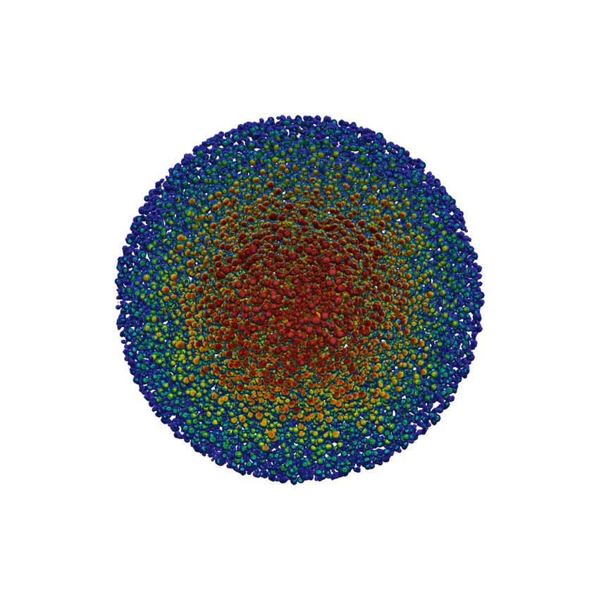
5.2. Saturation of cell aggregates under electroporation
The time evolution of the permeability in the cluster of cells is visualized in figure 15. Three
snapshots of the cluster are shown. These snapshots are color coded with the amount of perme-
ability (hotter colors) and present its distribution within the cluster environment. We find that the
permeability is very quickly saturated in the medium with higher values closer to the electrodes. An
effective penetration depth is also evident for the electropermeabilization of the cells in the cluster.
17Figure 15: Time evolution of the the cell membrane permeability in a cell cluster environment. Hotter
colors represent higher values of permeability. As observed, permeability enhances with time, reaching a
maximum saturation level after about half the simulation time. The dashed black line is the half-plane
cutting the spherical cluster, this is to demonstrate the internal structure of the cell aggregate permeability.
5.3. Impedance of the aggregate: a macro-level observable
In these simulations we apply a constant and uniform potential difference between the electrodes.
The electric field will adapt to the geometric configuration of the domain as well as the cells while
the cell membranes also distort the field. The distortions in the observed electric field close to the
boundaries, where the electrodes are located, produce a different profile for the “needle potential”
that the cluster experiences. Needle intensity is defined in equation 17. The needle intensity in our
simulation is shown in figure 16(a).
Z
I(t) = σ e ∂n V (t, x)ds, (17)
E
where E is one of the electrodes where the voltage is imposed.
Furthermore, one can measure the overall permeability within the environment by measuring
the impedance of the sample detected at the electrodes. We define the impedance of the cluster of
cells as:
R
V (t, x)dx
Z(t) = R E , (18)
E
σ∂n V (t, x)dx
The time evolution of impedance of the cluster of cells simulated here is shown in figure 16(b). A
strong negative correlation is observed between the impedance and the overall degree of permeabil-
ity. We also note that the exact magnitude of impedance and intensity felt at each electrode depends
on the distance of the north pole to the electrode. Here we show these results only qualitatively for
a distance of 0.01 × Rcluster .
We find that even though permeabilized cells have a huge increase of their membrane conduc-
tance (from 1 to 104 S/m2 ), as qualitatively illustrated in figure 15, the relative impedance of the
aggregate drops from 1 to 0.6.
18Figure 16: Time evolution of the needle intensity (left) as well as the resulting cluster impedance under a
constant external potential difference (right).
6. Conclusion
We have presented a computational framework for parallel simulations of cell aggregate electrop-
ermeabilization on a mesoscale cluster of cells. We used an adaptive Voronoi mesh along with a level
set method to represent the interfaces. We described the parallel strategy for this implementation.
The core aspects of our methodology are its efficiency and excellent scalability. Our tests indicate
excellent performance for large scale simulations for up to 4096 processors and physical tissue sizes
of a few cubic millimeters. Also, the Octree data structure has helped us to reduce the complexity
of the linear systems arising in our discretization by orders of magnitude. With this technique we
were able to discretize the farther domain at 29−2 = 128 times coarser than the finest grids adjacent
to the boundaries of the cells without loss of accuracy.
We emphasize that previously this phenomenon was simulated using serial approaches, which
were not able to go beyond micro-scale simulations. Hence, the main accomplishment of our imple-
mentation is that it empowers mesoscale simulations of cell aggregate electropermeabilization and
paves the way for a wide range of comparison with biological studies on cell aggregates. The present
manuscript provides preliminary numerical results on cell aggregates electropermeabilization which
qualitatively corroborate the experimental observations. In particular, the electroporated region of
the spheroids as given in figure 13 is in accordance with the experimental data of spheroid electro-
poration of Rols et al. [33]. Namely, as for cells, the electroporation of spheroids is the highest
at the pole. Moreover, thanks to our new computational framework, the multiscale understanding
of electroporation from the cell to the tissue is possible. For instance we plan to compare the
macroscopic experimental data (e.g. the tissue or spheroid impedances) with the corresponding
numerical quantities.
In order to push forward the comparison of the simulations with the experiments, it will be nec-
essary to add the mesoscale description of drug or DNA transport across the membranes, following
the recently proposed microscale model of Leguèbe et al. [15, 16]. We also aim to develop semi-
analytic models to mimic the mesoscale electropermeabilization of a cluster of cells. Our utmost
goal is to provide a computational tool for biologists to better study targeted drug delivery via un-
derstanding electropermeabilization physics as well as the transport mechanisms that consequently
aids cancer treatment.
19Acknowledgement
The research of P. Mistani, A. Guittet and F. Gibou was supported by NSF DMS-1412695
and ARO W911NF-16-1-0136. C. Poignard research is supported by Plan Cancer DYNAMO (ref.
PC201515) and Plan Cancer NUMEP (ref. PC201615). C.P.’s research is partly performed within
the scope of the European Associated Laboratory EBAM on electroporation, granted by CNRS. P.
Mistani would like to thank Daniil Bochkov for fruitful discussions that have contributed to this
research. This work used the Extreme Science and Engineering Discovery Environment (XSEDE),
which is supported by National Science Foundation grant number ACI-1053575. The authors ac-
knowledge the Texas Advanced Computing Center (TACC) at The University of Texas at Austin
for providing HPC and visualization resources that have contributed to the research results re-
ported within this paper. This research is performed within the scope of the Inria associate team
NUM4SEP, between the CASL group at UCSB and the Inria team MONC.
References
References
[1] M. Bedau. Downward causation and the autonomy of weak emergence. Principia, 6(1):5, 2002.
[2] E. Braaten and G. Weller. An improved low-discrepancy sequence for multidimensional quasi-
monte carlo integration. Journal of Computational Physics, 33(2):249 – 258, 1979.
[3] C. Burstedde, L. C. Wilcox, and O. Ghattas. p4est: Scalable algorithms for parallel adaptive
mesh refinement on forests of octrees. SIAM Journal on Scientific Computing, 33(3):1103–1133,
2011.
[4] K. A. DeBruin and W. Krassowska. Modeling electroporation in a single cell. i. effects of field
strength and rest potential. Biophysical Journal, 77(3):1213 – 1224, 1999.
[5] R. P. Fedkiw, T. Aslam, B. Merriman, and S. Osher. A non-oscillatory eulerian approach to
interfaces in multimaterial flows (the ghost fluid method). Journal of Computational Physics,
152(2):457 – 492, 1999.
[6] R. A. Finkel and J. L. Bentley. Quad trees a data structure for retrieval on composite keys.
Acta Informatica, 4(1):1–9, Mar 1974.
[7] C. A. Fulmer and C. Ostroff. Convergence and emergence in organizations: An integrative
framework and review. Journal of Organizational Behavior, 37(S1), 2016.
[8] F. Gibou, R. Fedkiw, and S. Osher. A review of level-set methods and some recent applications.
Journal of Computational Physics, 353(Supplement C):82 – 109, 2018.
[9] A. Guittet, M. Lepilliez, S. Tanguy, and F. Gibou. Solving elliptic problems with discontinu-
ities on irregular domains – the voronoi interface method. Journal of Computational Physics,
298:747 – 765, 2015.
[10] A. Guittet, C. Poignard, and F. Gibou. A voronoi interface approach to cell aggregate elec-
tropermeabilization. Journal of Computational Physics, 332:143–159, 2017.
[11] J. H. Halton. On the efficiency of certain quasi-random sequences of points in evaluating
multi-dimensional integrals. Numerische Mathematik, 2(1):84–90, Dec 1960.
[12] M. Kang, R. P. Fedkiw, and X.-D. Liu. A boundary condition capturing method for multiphase
incompressible flow. Journal of Scientific Computing, 15(3):323–360, Sep 2000.
[13] W. Krassowska and P. D. Filev. Modeling electroporation in a single cell. Biophysical Journal,
92(2):404 – 417, 2007.
20[14] J. Langus, M. Kranjc, B. Kos, T. Šuštar, and D. Miklavčič. Dynamic finite-element model for
efficient modelling of electric currents in electroporated tissue. 6:26409, may 2016.
[15] M. Leguèbe, A. Silve, L. Mir, and C. Poignard. Conducting and permeable states of cell
membrane submitted to high voltage pulses: Mathematical and numerical studies validated by
the experiments. Journal of Theoretical Biology, 2014.
[16] M. S. Leguèbe, M. G. Notarangelo, M. Twarogowska, R. Natalini, and C. Poignard. Mathe-
matical model for transport of DNA plasmids from the external medium up to the nucleus by
electroporation. Mathematical Biosciences, 285:1–13, Mar. 2017.
[17] G. Levy. An introduction to quasi-random numbers. Numerical Algorithms Group Ltd., 2002.
[18] J. Li and H. Lin. Numerical simulation of molecular uptake via electroporation. Bioelectro-
chemistry, 82(1):10 – 21, 2011.
[19] X.-D. Liu and T. Sideris. Convergence of the ghost fluid method for elliptic equations with
interfaces. Mathematics of computation, 72(244):1731–1746, 2003.
[20] J. McMahon, E. Signori, K. Wells, V. Fazio, and D. Wells. Optimisation of electrotransfer
of plasmid into skeletal muscle by pretreatment with hyaluronidase-increased expression with
reduced muscle damage. Gene therapy, 8(16):1264, 2001.
[21] D. Meagher. Geometric modeling using octree encoding. Computer Graphics and Image Pro-
cessing, 19(2):129 – 147, 1982.
[22] C. Min. Local level set method in high dimension and codimension. Journal of computational
physics, 200(1):368–382, 2004.
[23] C. Min and F. Gibou. Geometric integration over irregular domains with application to level
set methods. J. Comput. Phys., 226:1432–1443, 2007.
[24] C. Min and F. Gibou. A second order accurate level set method on non-graded adaptive
Cartesian grids. J. Comput. Phys., 225:300–321, 2007.
[25] M. Mirzadeh, A. Guittet, C. Burstedde, and F. Gibou. Parallel level-set methods on adaptive
tree-based grids. Journal of Computational Physics, 322:345 – 364, 2016.
[26] P. Mistani, A. Guittet, D. Bochkov, J. Schneider, D. Margetis, C. Ratsch, and F. Gibou. The
island dynamics model on parallel quadtree grids. Journal of Computational Physics, 2017.
[27] S. Osher and J. A. Sethian. Fronts propagating with curvature-dependent speed: Algorithms
based on hamilton-jacobi formulations. Journal of Computational Physics, 79(1):12 – 49, 1988.
[28] W. H. Press, S. A. Teukolsky, W. T. Vetterling, and B. P. Flannery. Numerical Recipes in
FORTRAN; The Art of Scientific Computing. Cambridge University Press, New York, NY,
USA, 2nd edition, 1993.
[29] G. Pucihar, T. Kotnik, J. Teissié, and D. Miklavčič. Electropermeabilization of dense cell
suspensions. European Biophysics Journal, 36(3):173–185, 2007.
[30] C. H. Rycroft. Voro++: A three-dimensional voronoi cell library in C++. Chaos: An Inter-
disciplinary Journal of Nonlinear Science, 19(4):041111, 2009.
[31] J. Strain. Tree methods for moving interfaces. Journal of Computational Physics, 151(2):616–
648, 1999.
[32] D. Voyer, A. Silve, L. M. Mir, R. Scorretti, and C. Poignard. Dynamical modeling of tissue
electroporation. Bioelectrochemistry, 119:98 – 110, 2018.
[33] L. Wasungu, J.-M. Escoffre, A. Valette, J. Teissie, and M.-P. Rols. A 3d in vitro spheroid model
as a way to study the mechanisms of electroporation. International Journal of Pharmaceutics,
379(2):278 – 284, 2009. Challenges for Nanotechnology in Delivery Imaging.
21You can also read