Planet formation: key mechanisms and global models
←
→
Page content transcription
If your browser does not render page correctly, please read the page content below
Planet formation: key mechanisms and global
                                               models

                                               Sean N. Raymond and Alessandro Morbidelli
arXiv:2002.05756v1 [astro-ph.EP] 13 Feb 2020

                                               Abstract
                                               Models of planet formation are built on underlying physical processes. In order to
                                               make sense of the origin of the planets we must first understand the origin of their
                                               building blocks.
                                               This review comes in two parts. The first part presents a detailed description of six
                                               key mechanisms of planet formation:
                                               •   The structure and evolution of protoplanetary disks
                                               •   The formation of planetesimals
                                               •   Accretion of protoplanets
                                               •   Orbital migration of growing planets
                                               •   Gas accretion and giant planet migration
                                               •   Resonance trapping during planet migration
                                               While this is not a comprehensive list, it includes processes for which our under-
                                               standing has changed in recent years or for which key uncertainties remain.
                                               The second part of this review shows how global models are built out of planet
                                               formation processes. We present global models to explain different populations of
                                               known planetary systems, including close-in small/low-mass planets (i.e., super-
                                               Earths), giant exoplanets, and the Solar System’s planets. We discuss the different
                                               sources of water on rocky exoplanets, and use cosmochemical measurements to
                                               constrain the origin of Earth’s water. We point out the successes and failings of
                                               different models and how they may be falsified.
                                               Finally, we lay out a path for the future trajectory of planet formation studies.

                                               Sean N. Raymond
                                               Laboratoire d’Astrophysique de Bordeaux, CNRS and Université de Bordeaux, Pessac, France
                                               e-mail: rayray.sean@gmail.com
                                               Alessandro Morbidelli
                                               Laboratoire Lagrange, Observatoire de la Cote d’Azur, Nice, France
                                               e-mail: morby@oca.eu

                                                                                                                                          1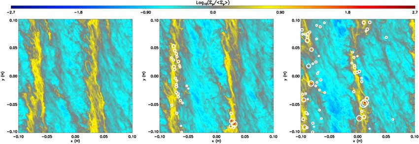
2 Sean N. Raymond and Alessandro Morbidelli
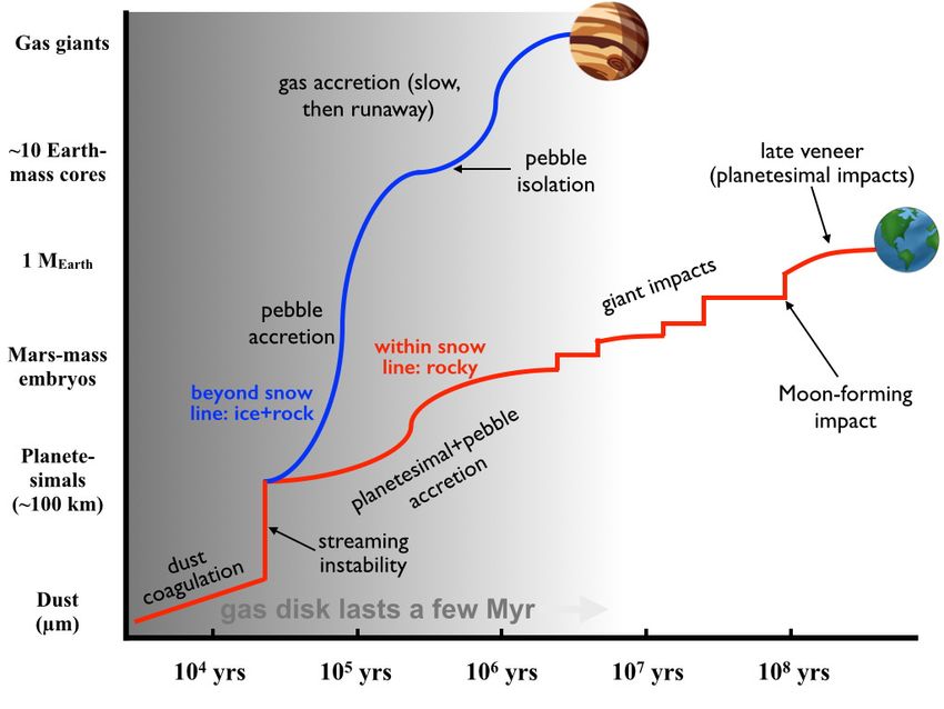
Fig. 1 Schematic view of some of the processes involved in forming Jupiter and Earth. This diagram
is designed to present a broad view of the relevant mechanisms but still does not show a number
of important effects. For instance, we know from the age distribution of primitive meteorites that
planetesimals in the Solar System formed in many generations, not all at the same time. In addition,
this diagram does not depict the large-scale migration thought to be ubiquitous among any planets
more massive than roughly an Earth-mass (see discussion in text). Adapted from [322].
1 Observational constraints on planet formation models
If planet building is akin to cooking, then a review of planet formation is a cookbook.
Planetary systems – like dishes – come in many shapes and sizes. Just as one cooking
method cannot produce all foods, a single growth history cannot explain all planets.
While the diversity of dishes reflects a range of cooking techniques and tools, they
are all drawn from a common set of cooking methods. Likewise, the diversity of
planetary systems can be explained by different combinations of processes drawn
from a common set of physical mechanisms. Our goal in this review is first to describe
the key processes of planet formation and then to show how they may be combined
to generate global models, or recipes, for different types of planetary systems.
To illustrate the processes involved, Fig. 1 shows a cartoon picture of our current
vision for the growth of Earth and Jupiter. Both planets are thought to have formed
from planetesimals in different parts of the Solar System. In our current understand-
ing, the growth tracks of these planets diverge during the pebble accretion process,
which is likely to be much more efficient past the snow line [254, 335]. There exists a
much larger diversity of planets than just Jupiter and Earth, and many vital processes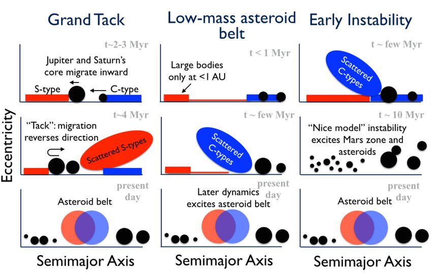
Planet formation: key mechanisms and global models                                              3

are not included in the Figure, yet it serves to illustrate how divergent formation
pathways can contribute to planetary diversity.
   We start this review by summarizing the key constraints on planet formation
models. Constraints come from Solar System measurements (e.g., meteorites), ob-
servations of other planetary systems (e.g., exoplanets and protoplanetary disks), as
well as laboratory measurements (e.g., to measure the sticking properties of small
grains).

Solar System Constraints

Centuries of human observation have generated a census of the Solar System, albeit
one that is still not 100% complete. The most important constraints for planet for-
mation include our system’s orbital architecture as well as compositional and timing
information gleaned from in-situ measurements. An important but challenging exer-
cise is to distill the multitude of existing constraints into just a few large-scale factors
to which resolution-limited models can be compared.
   The central Solar System constraints are:
• The masses and orbits of the terrestrial planets.1 The key quantities include
  their number, their absolute masses and mass ratios, and their low-eccentricity,
  low-inclination orbits. These have been quantified in studies that attempted to
  match their orbital distribution. For example the normalized angular momentum
  deficit AM D is defined as[260, 88]:
                                       √
                                                        q
                                Í                              2
                                  j m j a j 1 − cos(i j ) 1 − e j
                      AM D =                Í     √                 ,         (1)
                                              j mj aj

   where a j , e j , i j , and m j correspond to planet j’s semimajor axis, eccentricity,
   orbital inclination, and mass. The Solar System’s terrestrial planets have an AM D
   of 0.0018.
   The radial mass concentration statistic RMC (called Sc by [88]) is a measure of
   the radial mass profile of the planets. It is defined as:
                                                     Í
                                                        mj
                              RMC = max Í                               .            (2)
                                                m j [log10 (a/a j )]2

   The function in brackets is calculated sweeping a across all radii, and the RMC
   represents the maximum. For a one-planet system RMC is infinite. The RMC is
   higher when the planets’ masses are concentrated in narrow radial zones (as is
   the case in the terrestrial planets, with two large central planets and two small

1 The terms “terrestrial” and “rocky” planet are interchangeable: the Solar System community gen-
erally uses the term terrestrial and the exoplanet community uses rocky. We use both terminologies
in this review to represent planets with solid surfaces that are dominated (by mass) by rock and
iron.
4                                             Sean N. Raymond and Alessandro Morbidelli

  exterior ones). The RMC becomes smaller for systems that are more spread
  out and systems in which all planets have similar masses. The Solar System’s
  terrestrial planets’ RMC is 89.9.
  Confronting distributions of simulated planets with these empirical statistics (as
  well as other ones) has become a powerful and commonly-used discriminant of
  terrestrial planet formation models [88, 373, 428, 426, 423, 104, 291].
• The masses and orbits of the giant planets. As for the terrestrial planets, the
  number (two gas giant, two ice giant), masses and orbits of the giant planets are
  the central constraints. The orbital spacing of the planets is also important, for
  instance the fact that no pair of giant planets is located in mean motion resonance.
  An important, overarching factor is simply that the Solar System’s giant planets
  are located far from the Sun, well exterior to the orbits of the terrestrial planets.
• The orbital and compositional structure of the asteroid belt. While spread
  over a huge area the asteroid belt contains only ∼ 4.5 × 10⁻⁴ M ⊕ in total mass
  [246, 252, 125], orders of magnitude less than would be inferred from models
  of planet-forming disks such as the very simplistic minimum-mass solar nebula
  model [495, 189]. The orbits of the asteroids are excited, with eccentricities that
  are roughly evenly distribution from zero to 0.3 and inclinations evenly spread
  from zero to more than 20◦ (a rough stability limit given the orbits of the planets).
  While there are a number of compositional groups within the belt, the general
  trend is that the inner main belt is dominated by S-types and the outer main belt by
  C-types [171, 125, 126]. S-type asteroids are associated with ordinary chondrites,
  which are quite dry (with water contents less than 0.1% by mass), and C-types are
  linked with carbonaceous chondrites, some of which (CI, CM meteorites) contain
  ∼ 10% water by mass [436, 236, 10].
• The cosmochemically-constrained growth histories of rocky bodies in the
  inner Solar System. Isotopic chronometers have been used to constrain the ac-
  cretion timescales of different solid bodies in the Solar System. Ages are generally
  measured with respect to CAIs (Calcium and Aluminum-rich Inclusions), mm-
  sized inclusions in chondritic meteorites that are dated to be 4.568 Gyr old [67].
  Cosmochemical measurements indicate that chondrules, which are similar in size
  to CAIs, started to form at roughly the same time [107, 371]. Age dating of
  iron meteorites suggests that differentiated bodies – large planetesimals or plan-
  etary embryos – were formed in the inner Solar System within 1 Myr of CAIs
  [181, 251, 448]. Isotopic analyses of Martian meteorites show that Mars was fully
  formed within 5-10 Myr after CAIs [368, 117], whereas similar analyses of Earth
  rocks suggest that Earth’s accretion did not finish until much later, roughly 100
  Myr after CAIs [476, 240].
  There is evidence that two populations of isotopically-distinct chondritic me-
  teorites – the so-called carbonaceous and non-carbonaceous meteorites – have
  similar age distributions [250]. Given that chondrules are expected to undergo
  very fast radial drift within the disk [494, 253], this suggests that the two pop-
  ulations were kept apart and radially segregated, perhaps by the early growth of
  Jupiter’s core [250].
Planet formation: key mechanisms and global models                                   5

Constraints from Observations of Planet-forming disks around other stars

Gas-dominated protoplanetary disks are the birthplaces of planets. Disks’ structure
and evolution plays a central role in numerous processes such as how dust drifts
[47], where planetesimals form [135, 134], and what direction and how fast planets
migrate [51].
   We briefly summarize the main observational constraints from protoplanetary
disks for planet formation models (see also dedicated reviews [506, 25, 11]):
• Disk lifetime. In young clusters virtually all stars have detectable hot dust, which
  is used as a tracer for the presence of gaseous disks [179, 70]. However, in
  old clusters very few stars have detectable disks. Analyses of a large number of
  clusters of different ages indicate that the typical timescale for disks to dissipate
  is a few Myr [179, 70, 192, 294, 390]. Fig. 2 shows this trend, with the fraction
  of stars with disks decreasing as a function of cluster age. It is worth noting that
  observational biases are at play, as the selection of stars that are members of
  clusters can affect the interpreted disk dissipation timescale [392].
• Disk masses. Most masses of protoplanetary disks are measured using sub-mm
  observations of the outer parts of the disk in which the emission is thought to be
  optically thin [506]. Disk masses are commonly found to be roughly equivalent to
  1% of the stellar mass, albeit with a 1-2 order of magnitude spread [140, 17, 18,
  21, 506]. It has recently been pointed out that there is tension between the inferred
  disk masses and the masses of exoplanet systems, as a large fraction of disks do
  not appear to contain enough mass to produce exoplanet systems [295, 352], even
  assuming a very high efficiency of planet formation (see Fig. 2).
• Disk structure and evolution. ALMA observations suggest that disks are typ-
  ically 10-100 au in scale [36], similar to the expected dimensions of the Sun’s
  protoplanetary disk [189, 168, 247]. Sub-mm observations at different radii in-
  dicate that the surface density of dust Σ in the outer parts of disks follows a
  roughly Σ ∼ r −1 radial surface density slope [353, 287, 19, 20], consistent with
  simple models for accretion disks. Many disks observed with ALMA show ringed
  substructure [14, 22, 16]. Disks are thought to evolve by accreting onto their host
  stars, and the accretion rate itself has been measured to vary as a function of
  time; indeed, the accretion rate is often used as a proxy for disk age [185, 25]. As
  disks age, they evaporate from the inside-out by radiation from the central star
  [12, 382, 11] and, depending on the stellar environment, may also evaporate from
  the outside-in due to external irradiation [194, 4].
• Dust around older stars. Older stars with no more gas disks often have observable
  dust, called debris disks (recent reviews: [315, 200]). Roughly 20% of Sun-like
  stars are found to have dust at mid-infrared wavelengths [74, 478, 329]. This dust is
  thought to be associated with the slow collisional evolution of outer planetesimal
  belts akin to our Kuiper belt but generally containing much more mass [515, 248].
  The occurrence rate of dust is observed to decrease with the stellar age [324, 79].
  More [less] massive stars have significantly higher [lower] occurrence of debris
  disks [463, 268]. There is no clear observed correlation between debris disks and
  planets [347, 300, 348]. A significant fraction of old stars have been found to
6                                                   Sean N. Raymond and Alessandro Morbidelli

Fig. 2 Two observational constraints on planet-forming disks. Left: The fraction of stars that
have detectable disks in clusters of different ages. This suggests that the typical gaseous planet-
forming disk only lasts a few Myr [179, 70, 192]. From [294]. Right: A comparison between
inferred disk masses and the mass in planets in different systems, as a function of host star mass.
The dust mass (red) is measured using sub-mm observations (and making the assumption that
the emission is optically thin), and the gas mass is inferred by imposing a 100:1 gas to dust
ratio. There is considerable tension, as the population of disks does not appear massive enough
to act as the precursors of the population of known planets. The solution to this problem is not
immediately obvious. Perhaps disk masses are systematically underestimated [172], or perhaps
disks are continuously re-supplied with material from within their birth clusters via Bondi-Hoyle
accretion [473, 327]. From [295].

    have warm or hot exo-zodiacal dust [2, 142, 245]. The origin of this dust remains
    mysterious as there is no clear correlation between the presence of cold and hot
    dust [142].

Constraints from Extra-Solar Planets

With a catalog of thousands of known exoplanets, the constraints from planets around
other stars are extremely rich and constantly being improved. Figure 3 shows the
orbital architecture of a (non-representative) selection of known exoplanet systems.
While there exist biases in the detection methods used to find exoplanets [508], their
sheer number form the basis of a statistical framework with which to confront planet
formation theories.
   We can grossly summarize the exoplanet constraints as follows:
• Occurrence and demographics. Over the past few decades it has been shown
  using multiple techniques that exoplanets are essentially ubiquitous [318, 85, 38].
  Despite the observational biases, a huge diversity of planetary systems has been
  discovered. Yet when drawing analogies with the Solar System, it is worth noting
  that, if our Sun were to have been observed with present-day technology Jupiter
  is the only planet that could have been detected [339, 422]. This makes the
  Solar System unusual at roughly the1% level. In addition, the Solar System is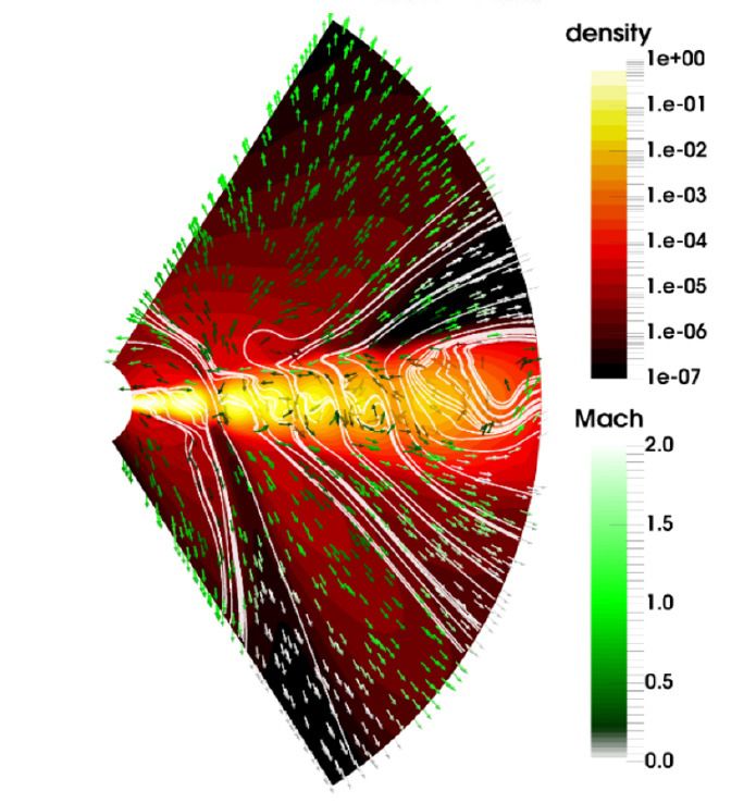
Planet formation: key mechanisms and global models                                                       7

                                                              Transiting Systems
            Kepler-79
           Kepler-444
           Kepler-402
           Kepler-299
           Kepler-292
           Kepler-265
            Kepler-24
           Kepler-172
           Kepler-150
           Kepler-122
           Kepler-107
            Kepler-36
            Kepler-90
           Kepler-223
            Kepler-11
           Kepler-296
           Kepler-186
            Kepler-33
            WASP-47
         TRAPPIST-1
                                                              RV-detected Systems
            GJ 667 C
            HD 69830
          HD 168443
              51 Peg
            HD 79498
            HD 40307
             ups And
              GJ 876
              55 Cnc

        Solar System

                  0.01                   0.10         1.00                               10.00
                                        Semimajor Axis (AU)

Fig. 3 A sample of exoplanet systems selected by hand to illustrate their diversity (from [422]). The
systems at the top were discovered by the transit method and the bottom systems by radial velocity
(RV). Of course, some planetsare detected in both transit and RV (e.g. 55 Cnc e; [127]). A planet’s
size is proportional to its actual size (but is not to scale on the x-axis). For RV planets without transit
detections we used the M sini ∝ R2.06 scaling derived by [284]. For giant planets (M > 50 M⊕ )
on eccentric orbits (e > 0.1; also for Jupiter and Saturn), the horizontal error bar represents the
planet’s pericenter to apocenter orbital excursion. The central stars vary in mass and luminosity;
e.g., TRAPPIST-1 is an ultracool dwarf star with mass of only 0.08 M [162]. A handful of systems
have ∼Earth-sized planets in their star’s habitable zones, such as Kepler-186 [407], TRAPPIST-
1 [162], and GJ 667 C [24]. Some planetary systems – for example, 55 Cancri [146] – are found in
multiple star systems.
8                                             Sean N. Raymond and Alessandro Morbidelli

  borderline unusual in not containing any close-in low-mass planets [302, 352].
  For the purposes of this review we focus on two categories of planets: gas giants
  and close-in low-mass planets, made up of high-density ‘super-Earths’ and puffy
  ‘mini-Neptunes’.
• Gas giant planets: occurrence and orbital distribution. Radial velocity surveys
  have found giant planets to exist around roughly 10% of Sun-like stars [113, 318].
  Roughly one percent of Sun-like stars have hot Jupiters on very short-period orbits
  [196, 512], very few have warm Jupiters with orbital radii of up to 0.5-1 au [77,
  481], and the occurrence of giant planets increases strongly and plateaus between
  1 to several au, and there are hints that it decreases again farther out [318, 145];
  see Fig. 16. Direct imaging surveys have found a dearth of giant planets on wide-
  period orbits, although only massive young planets tend to be detectable [68].
  Microlensing surveys find a similar overall abundance of gas giants as radial
  velocity surveys and have shown that ice giant-mass planets appear to be far more
  common than their gas giant counterparts [170, 464]. Giant planet occurrence
  has also been shown to be a strong function of stellar metallicity, with higher
  metallicity stars hosting many more giant planets [169, 443, 261, 147, 121].
• Close-in low-mass planets: occurrence and orbital distribution. Perhaps the
  most striking exoplanet discovery of the past decade was the amazing abundance
  of close-in small planets. Planets between roughly Earth and Neptune in size or
  mass with orbital periods shorter than 100 days have been shown to exist around
  roughly 30-50% of all main sequence stars [318, 195, 157, 131, 391, 508]. Both
  the masses and radii have been measured for a subset of planets [297] and analyses
  have shown that the smaller planets tend to have high densities and the larger ones
  have low densities, which has been interpreted as a transition between rocky
  ‘super-Earths’ and gas-rich ‘mini-Neptunes’ with a transition size or mass of
  roughly 1.5−2 R ⊕ or ∼ 3−5 M ⊕ [499, 497, 437, 511, 97]. For the purposes of this
  review we generally lump together all close-in planets smaller than Neptune and
  call them super-Earths for simplicity. The super-Earth population has a number
  of intriguing characteristics that constrain planet formation models. While they
  span a range of sizes, within a given system super-Earths tens to have very similar
  sizes [325, 498]. Their period ratios form a broad distribution and do not cluster at
  mean motion resonances[284, 143]. Finally, in the Kepler survey the majority of
  super-Earth systems only contain a single super-Earth [38, 440], which contrasts
  with the high-multiplicity rate found in radial velocity surveys [318].

Outline of this review

The rest of this chapter is structured as follows.
   In Section 2 we will describe six essential mechanisms of planet formation. These
are:
• The structure and evolution of protoplanetary disks (Section 2.1)
• The formation of planetesimals (Section 2.2)
• Accretion of protoplanets (Section 2.3)
Planet formation: key mechanisms and global models                                      9

• Orbital migration of growing planets (Section 2.4)
• Gas accretion and giant planet migration (Section 2.5)
• Resonance trapping during planet migration (Section 2.6)
This list does not include every process related to planet formation. These processes
have been selected because they are both important and are areas of active study.
    Next we will build global models of planet formation from these processes (Sec-
tion 3). We will first focus on models to match the intriguing population of close-in
small/low-mass planets: the super-Earths (Section 3.1). Next we will turn our at-
tention to the population of giant planets, using the population of known giant
exoplanets to guide our thinking about the formation of our Solar System’s giant
planets (Section 3.2). Next we will turn our attention to matching the Solar System
itself (Section 3.3), starting from the classical model of terrestrial planet formation
(Section 3.3.1) and then discussing newer ideas: the Grand Tack (Section 3.3.2),
Low-mass Asteroid belt (Section 3.3.3) and Early Instability (Section 3.3.4) models.
Then we will discuss the different sources of water on rocky exoplanets, and use
cosmochemical measurements to constrain the origin of Earth’s water (Section 3.4).
Finally, in Section 4 we will lay out a path for the future trajectory of planet formation
studies.

2 Key processes in planet formation

In this Section we review basic properties that affect the disk’s structure, planetesi-
mals and planet formation as well as dynamical evolution. These processes build the
skeleton of our understanding of how planetary systems are formed. As pieces of a
puzzle, they will then be put together to develop models on the origin of the different
observed structures of planetary systems in Sec. 3.

2.1 Protoplanetary disks: structure and evolution

Planet formation takes place in gas-dominated disks around young stars. These disks
were inferred by Laplace [259] from the near-perfect coplanarity of the orbits of
the planets of the Solar System and of angular momentum conservation during
the process of contraction of gas towards the central star. Disks are now routinely
observed (imaged directly or deduced through the infrared excess in the spectral
energy distribution) around young stars. The largest among protoplanetary disks are
now resolved by the ALMA mm-interferometer ([16]). Here we briefly review the
viscous-disk model and the wind-dominated model. For more in depth reading we
recommend [25] and [480].
10                                              Sean N. Raymond and Alessandro Morbidelli

2.1.1 Viscous-disk model(s)

The simplest model of a protoplanetary disk is a donut of gas and dust in rotation
around the central star evolving under the effect of its internal viscosity. This is
hereafter dubbed the viscous-disk model. Because of Keplerian shear, different rings
of the disk rotate with different angular velocities, depending on their distance from
the star. Consequently, friction is exerted between adjacent rings. The inner ring,
rotating faster, tends to accelerate the outer ring (i.e. it exerts a positive torque) and
the outer ring tends to decelerate the inner ring (i.e. exerting a negative torque of
equal absolute strength). It can be demonstrated (see for instance [178]) that such a
torque is
                                     T = 3πΣνr 2 Ω ,                                    (3)
where Σ is the surface density of the disk at the bounday between the two rings, ν is
the viscosity, and Ω is the rotational frequency at the distance r from the star.
   A fundamental assumption of a viscous-disk model is that it is in steady state,
which means the the mass flow of gas MÛ is the same at any distance r. Under this
assumption it can be demonstrated that the gas flows inwards with a radial speed
                                                3ν
                                       vr = −                                          (4)
                                                2r
and that the product νΣ is independent of r. That is, the radial dependence of Σ is the
inverse of the radial dependence of ν. Of course the steady-state assumption is valid
only in an infinite disk. In a more realistic disk with a finite size, this assumption
is good only in the inner part of the disk, whereas the outer part expands into the
vacuum under the effect of the viscous torque [292].
   If viscosity rules the radial structure of the disk, pressure rules the vertical struc-
ture. At steady state, the disk has to be in hydrostatic equilibrium, which means that
the vertical component of the gravitational force exerted by the star has to be equal
and opposite to the pressure force, i.e.:

                                    GM∗     1 dP
                                        z=−      ,                                     (5)
                                     r3     ρ dz
where M∗ is the mass of the star, z is the height over the disk’s midplane, ρ is
the volume density of the disk and P is its pressure. Using the perfect gas law
P = R/ρT/µ (where R is the gas constant, µ is the molecular weight of the gas and
T is the temperature) and assuming that the gas is vertically isothermal (i.e. T is a
function of r only), equation (5 gives the solution:

                                                  z2

                              ρ(z) = ρ(0) exp − 2 ,                               (6)
                                                 2H
             p
where H = Rr 3T/µ is called the pressure scale-height of the disk (the gas extends
to several scale-heights, with exponentially vanishing density).
Planet formation: key mechanisms and global models 11
We now need to compute T(r). The simplest way is to assume that the disk is solely
heated by the radiation from the central star (passive disk assumption, see [100]).
Most of the disk is opaque to radiation, so the star can illuminate and deposit heat
only on the surface layer of the disk, here defined as the layer where the integrated
optical depth along a stellar ray reaches unity. For simplicity we assume that the
stellar radiation hits a hard surface, whose height over the midplane is proportional
to the pressure scale-height H. Then, the energy deposited on this surface between
r and r + δr from the star is:
L∗
E+Irr = (2πr)(rδh) , (7)
4πr 2
where δh is the change in aspect ratio H/r over the range δr, namely d(H/r)/drδr;
the parentheses have been put in (7) to regroup the terms corresponding respectively
to (i) stellar brightness L∗ at distance r, (ii) circumference of the ring and (iii)
projection of H(r + δr) − H(r) on the direction orthogonal to the stellar ray hitting
the surface. On the other had, the same surface will cool by black-body radiation in
space at a rate
E−Irr = 2πrδrσT 4 (8)
where σ is Boltzman’s constant. Equating (7) and (8) and remembering the definition
of H as a function of r and T leads to
T(r) ∝ r −3/7 and H/r ∝ r 2/7 . (9)
The positive exponent in the dependence of the aspect ratio H/r on r implies that
the disk is flared. Notice that neither quantities in Eq. 9 depend on disk’s surface
density, opacity or viscosity.
However, because we are dealing with a viscous disk, we cannot neglect the heat
released by viscous dissipation, i.e. in the friction between adjacent rings rotating at
different speeds. Over a radial width δr, this friction dissipates energy at a rate ([25]
9
E+V isc = ΣνΩ2 2πrδr . (10)
8
This heat is dissipated mostly close to the midplane, where the disk’s volume density
is highest. This changes the cooling with respect to Eq. 8. The energy cannot be
freely irradiated in space; it has first to be transported from the midplane through the
disk, which is opaque to radiation, to the “surface” boundary with the optically thin
layer. Thus the cooling term in Eq. 8 has to be divided by κΣ, where κ is the disk’s
opacity. Again by balancing heating and cooling and the definition of H we find:
H/r ∝ ( MÛ 2 κ/νr)1/8 , (11)
where we have used that MÛ = 2πrvr Σ = −3πνΣ.
To know the actual radial dependence of this expression, we need to know the
radial dependences of κ and ν (remember that MÛ is assumed to be independent of r).12 Sean N. Raymond and Alessandro Morbidelli
The opacity depends on temperature, hence on r in a complicated manner, with abrupt
transitions when the main chemical species (notably water) condense [43]. Let’s
ignore this for the moment. Concerning ν(r), Shakura and Sunyaev [454] proposed
from dimensional analysis that the viscosity is proportional to the square of the
characteristic length of the system and is inversely proportional to the characteristic
timescale. At a distance r from the star, the characteristic length of a disk is H(r)
and the characteristic timescale is the inverse of the orbital frequency Ω. Thus they
postulated ν = αH 2 Ω, where α is an unknown coefficient of proportionality. If one
adopts this prescription for the viscosity, the viscous-disk model is qualified as an
α-disk model. Injecting this definition of ν into Eq. 11 one obtains
1/10
κ MÛ 2
H/r ∝ r 1/20 . (12)
α
This result implies that the aspect ratio of a viscously heated disk is basically
independent of r (and T ∝ 1/r), in sharp contrast with the aspect ratio of a passive
disk. Because the disk is both heated by viscosity and illuminated by the star, its
aspect ratio at each r will be the maximum between Eq. 12 and Eq. 9: it will be flat
in the inner part and flared in the outer part. Because Eq. 12 depends on opacity,
accretion rate and α, the transition from the flat disk and the flared disk will depend
on these quantities. In particular, given that MÛ decreases with time as the disk is
consumed by accretion of gas onto the star [185], this transition moves towards the
star as time progresses [51]. The effects of non-constant opacity introduce wiggles
of H/r over this general trend [51].
The viscous disk model is simple and neat, but its limitation is in the understanding
of the origin of the disk’s viscosity. The molecular viscosity of the gas is by orders of
magnitude insufficient to deliver the observed accretion rate MÛ onto the central star
[185] given a reasonable disk’s density, comparable to that of the Minimum Mass
Solar Nebula model (MMSN: [495], [189]). It was thought that the main source of
viscosity is turbulence and that turbulence was generated by the magneto-rotational
instability (see [34]). But this instability requires a relatively high ionization of the
gas, which is prevented when grains condense in abundance, at a temperature below
∼ 1, 000K [128]. Thus, only the very inner part of the disk is expected to be turbulent
and have a high viscosity. Beyond the condensation line of silicates, the viscosity
should be much lower. Remembering that νΣ has to be constant with radius, the
drop of ν at the silicate line implies an abrupt increase of Σ. As we will see, this
property has an important role in the drift of dust and the migration of planets. It
was expected that near the surface of the disk, where the gas is optically thin and
radiation from the star can efficiently penetrate, enough inoization may be produced
to sustain the Magneto Rotational Instability (MRI) [462]. However, these low-
density regions are also prone to other effects of non-ideal magneto-hydrodynamics
(MHD), like ambipolar diffusion and the Hall effect [32], which are expected to
quench turbulence. Thus, turbulent viscosity does not seem to be large enough
beyond the silicate condensation line to explain the stellar accretion rates that arePlanet formation: key mechanisms and global models 13
observed. This has promoted an alternative model of disk structure and evolution,
dominated by the existence of disk winds, as we review next.
2.1.2 Wind-dominated disk models
Unlike viscous disk models, which can be treated with simple analytic formulae,
the emergence of disk winds and their effects are consequence of non-ideal MHD.
Thus their mathematical treatment is complicated and the results can be unveiled only
through numerical simulations. Thus, this Section will remain at a phenomenological
level. For an in-depth study we recommend [32, 31, 480].
As we have seen above, the ionized regions of the disk have necessarily a low
density. If the disk is crossed by a magnetic field, the ions atoms in these low-density
regions can travel along the magnetic field lines without suffering collision with
neutral molecules. This is the essence of ambipolar diffusion.
Consider a frame co-rotating with the disk at radius r0 from the central star. In
this frame, fluid parcels feel an effective potential combining the gravitational and
centrifugal potentials. If poloidal (r, z) magnetic field lines act as rigid wires for fluid
parcels (which happens as long as the poloidal flow is slower than the local Alfven
speed)2, then a parcel initially at rest at r = r0 can undergo a runaway if the field
line to which it is attached is more inclined than a critical angle. Along such a field
line, the effective potential decreases with distance, leading to an acceleration of
magnetocentrifugal origin. This yields the inclination angle criterion θ > 30◦ for the
disk-surface poloidal field with respect to the vertical direction. Here fluid parcels
rotate at constant angular velocity and so increase their specific angular momentum.
Angular momentum is thus extracted from the disk and transferred to the ejected
material. As the disk loses angular momentum, some material has to be transferred
towards the central star, driving the stellar accretion. The efficiency of this process is
directly connected to the disk’s magnetic field strength, with a stronger field leading
to faster accretion.
In wind-dominated disk models the viscosity can be very low and the disk’s
density can be of the order of that of the MMSN. The observed accretion rate onto
the central star is not due to viscosity (the small value of νΣ provides only a minor
contribution) but is provided by the radial, fast advection of a small amount of
gas, typically at 3-4 pressure scale heights H above the disk’s midplane [174]. The
global structure of the disk can be symmetric (Fig. 4a) or asymmetric (Fig. 4b)
depending on simulation parameters and the inclusion of different physical effects
(e.g. the Hall effect). The origin of the asymmetry is not fully understood. In some
cases, the magnetic field lines can be concentrated in narrow radial bands that can
fragment the disk into concentric rings ([46]; see Fig. 4b). This effect is intriguing in
√
2 The Alfven speed is defined as the ratio between the magnetic field intensity B and µ0 ρ, where
µ0 is the permeability of vacuum and ρ is the total mass density of the charged plasma particles.
Apart from relativity effects, the Alfven speed is the phase speed of the Alfven wave, which is a
magnetohydrodynamic wave in which ions oscillate in response to a restoring force provided by an
effective tension on the magnetic field lines.14 Sean N. Raymond and Alessandro Morbidelli
light of the recent ALMA observations of the ringed structure of protoplanetary disks
[14, 22, 16]. It should be stressed, however, that there is currently no consensus on the
origin of the observed rings. An alternative possibility is that they are the consequence
of planet formation [521] or of other disk instabilities [474]. Understanding whether
ring formation in protoplanetary disks is a prerequisite for, or a consequence of,
planet formation is an essential goal of current research.
Depending on assumptions on the radial gradient of the magnetic field, and hence
of the strength of the wind, the gas density of the disk may be partially depleted
in its inner part [465] or preserve a global power-law structure similar to that of
viscous-disk models [30] (see Fig. 5). A positive surface density gradient as in
[465] has implication for the radial drift of dust and planetesimals [377] and for the
migration of protoplanets [376]. In addition in [465] the maximum of the surface
density (where dust and migrating planets tend to accumulate) moves outwards as
time progresses and the disk evolves.
Disk winds do not generate an appreciable amount of heat. In wind-dominated
models the disk temperature is close to that of a passive disk [343, 87], which has
a snowline inward of 1 au [51]. The deficit of water in inner solar system bodies
(the terrestrial planets and the parent bodies of enstatite and ordinary chondrites)
demonstrates that the protoplanetary solar disk inwards of 2-3 au was warm, at least
initially [333]. This implies that either the viscosity of the disk was quite high or
another form of heating – for instance the adiabatic compression of gas as it fell onto
the disk from the interstellar medium – was operating early on.
2.1.3 Dust dynamics
The dynamics of dust particles is largely driven by gas drag. Any time that there is a
difference in velocity between the gas and the particle, a drag force is exerted on the
particle which tends to erase the velocity difference. The friction time t f is defined as
the coefficient which relates the accelerations felt by the particle to the gas-particle
velocity difference, namely:
1
vÛ = − (v − u) , (13)
tf
where v is the particle velocity vector and u is the gas velocity vector, while vÛ is the
particle’s acceleration. The smaller a dust particle the shorter its t f . In the Epstein
regime, where the particle size is smaller than the mean free path of a gas molecule,
t f is linearly proportional to the particle’s size R. In the Stokes regime the particle
√
size is larger than the mean free path of a gas molecule and t f ∝ R. It is convenient
to introduce a dimensionless number, called the Stokes number, defined as τs = Ωt f ,
which represents the ratio between the friction time and the orbital timescale.
The effects of gas drag are mainly the sedimentation of dust towards the midplane
and its radial drift towards pressure maxima.
To describe an orbiting particle as it settles in a disk, cylindrical coordinates are
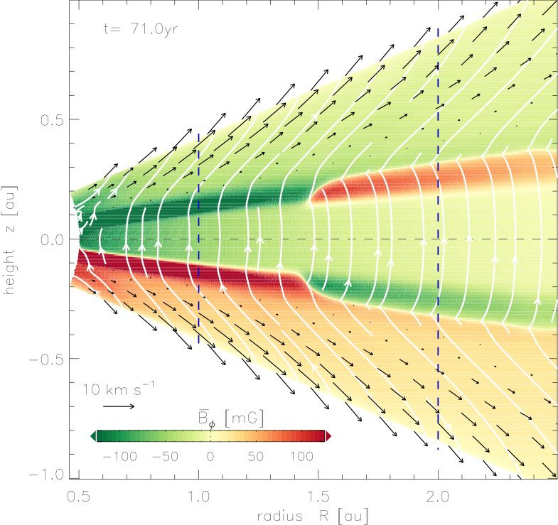
the natural choice. The stellar gravitational force can be decomposed into a radialPlanet formation: key mechanisms and global models 15 Fig. 4 Disk structure in two different wind-dominated disk global models. In the top panel from [174] shows the intensity and polarity of the magnetic field, the field lines and the velocity vectors of the wind. This disk model is symmetric relative to the mid-plane (anti-symmetric in polarity). The bottom panel from [46] shows the gas density, the magnetic field lines and the wind velocity vectors. This model has no symmetry relative to the midplane. Moreover, the disk is fragmented in rings by the accumulation of magnetic field lines in specific radial intervals.
16                                               Sean N. Raymond and Alessandro Morbidelli

Fig. 5 Comparison between the radial surface density distribution of the wind-dominated disk
models of ([465]), ([30]) and an α-disk model.

and a vertical component. The radial component is cancelled by the centrifugal
force due to the orbital motion. The vertical component, Fg,z = −mΩ2 z, where
m is the mass of the particle and z its vertical coordinate, instead accelerates the
particle towards the midplane, until its velocity vsettle is such that the gas drag force
FD = mvsettle /t f cancels Fg,z . This sets vsettle = Ω2 zt f and gives a settling time
Tsettle = z/vsettle = 1/(Ω2 t f ) = 1/(Ωτs ). Thus, for a particle with Stokes number
τs = 1 the settling time is the orbital timescale. However, turbulence in the disk
stirs up the particle layer, which therefore has a finite thickness. Assuming an α-disk
model, the scale height of the particle layer is [99]:
                                           H
                                   Hp = p          .                                   (14)
                                         1 + τs /α

   Dust particles undergo radial drift due to a small difference of their orbital velocity
relative to the gas. The gas feels the gravity of the central star and its own pressure.
The pressure radial gradient exerts a force Fr = −(1/ρ)dP/dr which can oppose or
enhance the gravitational force. As we saw above, P ∝ ρT, and ρ ∼ Σ/H. Because
Σ and T in general decrease with r, dP/dr < 0. The pressure force opposes to the
gravity force, diminishing it. Consequently, the gas parcels orbit the star at a speed
Planet formation: key mechanisms and global models 17
that is slightly slower than the Keplerian speed at the same location. The difference
between the Keplerian speed vk and the gas orbital speed is ηvK , where
2
1 H d log P
η=− (15)
2 r d log r
The radial velocity of a particle is then:
vr = −2ηvK τs /(τs2 − 1) + ur /(τs2 − 1) , (16)
where ur is the radial component of the gas velocity. Except for extreme cases ur is
very small and hence the second term in the right-hand side of Eq. 16 is negligible
relative to the first term. Consequently, the direction of the radial drift of dust depends
on the sign of η, i.e., from Eq. 15, on the sign of the pressure gradient. If the gradient
is negative as in most parts of the disk, the drift is inwards. But in the special regions
where the pressure gradient is positive, the particle’s drift is outwards. Consequently,
dust tends to accumulate at pressure maxima in the disk. We have seen above that
the MHD dynamics in the disk can create a sequence of rings and gaps, where the
density is alternatively maximal and minimal (Fig. 4b). Each of these rings therefore
features a pressure maximum along a circle. In absence of diffusive motion, the dust
would form an infinitely thin ring at the pressure maximum. Turbulence produces
diffusion of the dust particles in the radial direction, as it does in the vertical direction.
Thus, as dust sedimentation produces a layer with thicknesspgiven by Eq. 14, dust
migration produces a ring with radial thickness w p = w/ 1 + τs /α around the
pressure maximum, where w is the width of the gas ring assuming that it has a
Gaussian profile [138].
Consequently, observations of the dust distribution in protoplanetary disks can
provide information on the turbulence in the disk. The fact that the width of the gaps
in the disk of HL Tau appears to be independent of the azimuth despite the fact that
the disk is viewed with an angle smaller than 90◦ , suggests that the vertical diffusion
of dust is very limited such that α in Eq. 14 must be be 10−4 or less [399]. In contrast,
the observation that dust is quite broadly distributed in each ring of the disks, suggest
that α could be as large as 10−3 , depending on the particles Stokes number τs , which
is not precisely known [138]. These observations therefore suggest that turbulence
in the disks is such that the vertical diffusion it produces is weaker than the radial
diffusion. It is yet unclear which mechanism could generate turbulence with this
property.
2.2 Planetesimal formation
Dust particles orbiting within a disk often collide. If collisions are sufficiently gentle,
they stick through electrostatic forces, forming larger particles [57]. One could
imagine that this process continues indefinitely, eventually forming macroscopic
bodies called planetesimals. However, as we have seen above, particles drift through18 Sean N. Raymond and Alessandro Morbidelli
5
10
4
10
3
10
2
10
grain size [cm]
1 F
10
0
10 E
−1
10
−2
10
MT
−3 B
10
S SB
−4
10 −4 −3 −2 −1 0 1 2 3 4 5
10 10 10 10 10 10 10 10 10 10
grain size [cm]
Fig. 6 Map of collisional outcome in the disk. The sizes of colliding particles are reported on the
axes. The colours denote the result of each pair-wise collision. Green denotes growth, red denotes
erosion and yellow denotes neither of the above (i.e. a bounce). The label S stands for sticking, SB
for stick and bounce, B for bounce, MT for mass transfer, E for erosion and F for fragmentation.
Form ([507]). This map is computed for compact (silicate) particles, at 3 au.
the disk at different speeds depending on their size (or Stokes number). Thus, there is
a minimum speed at which particles of different sizes can collide. Particles of equal
size also have a distribution of impact velocities due to turbulent diffusion.
Fig. 6 shows a map of the outcome of dust collisions within a simple disk model,
from [507]. Using laboratory experiments on the fate of collisions as a function of
particle sizes and mutual velocities, and considering a disk with turbulent diffusion
α = 10−3 and drift velocities as in a MMSN disk, Windmark et al. computed the
growth/disruption maps for different heliocentric distances. The one from Fig. 6 is
for a distance of 3 au. The figure shows that, in the inner part of the disk, particles
cannot easily grow beyond a millimeter in size. A bouncing barrier prevents particles
to grow beyond this limit. If a particle somehow managed to grow to ∼ 10cm, itsPlanet formation: key mechanisms and global models 19
growth could potentially resume by accreting tiny particles. But as soon as particles
of comparable sizes hit each other, erosion or catastrophic fragmentation occurs,
thus preventing the formation of planetesimal-size objects.
The situation is no better in the outer parts of the disk. In the colder regions, due
to the lower velocities and the sticking effect of water ice, particles can grow to larger
sizes. But this size is nevertheless limited to a few centimeters due to the so-called
drift barrier (i.e. large enough particles start drifting faster than they grow: [47]).
It has been proposed that if particles are very porous, they could absorb better the
collisional energy, thus continuing to grow without bouncing or breaking [380]. Very
porous planetesimals could in principle form this way and their low densities would
make them drift very slowly through the disk. But eventually these planetesimals
would become compact under the effect of their own gravity and of the ram pressure
of the flowing gas [235]. This formation mechanism for planetesimals is still not
generally accepted in the community. At best, it could work only in the outer part of
the disk, where icy monomers have the tendency to form very porous structures, but
not in the inner part of the disk, dominated by silicate particles. Moreover, meteorites
show that the interior structure of asteroids is made mostly of compact particles of
100 microns to a millimeter in size, called chondrules, which is not consistent with
the porous formation mode.
A mechanism called the streaming instability [518] can bypass these growth bot-
tlenecks to form planetesimals. Although originally found to be a linear instability
(see [219]), this instability raises even more powerful effects which can be qualita-
tively explained as follows. This instability arises from the speed difference between
gas and solid particles. As the differential makes particles feel drag, the friction
exerted from the particles back onto the gas accelerates the gas toward the local
Keplerian speed. If there is a small overdensity of particles, the local gas is in a less
sub-Keplerian rotation than elsewhere; this in turn reduces the local headwind on
the particles, which therefore drift more slowly towards the star. Consequently, an
isolated particle located farther away in the disc, feeling a stronger headwind and
drifting faster towards the star, eventually joins this overdense region. This enhances
the local density of particles and reduces further its radial drift. This process drives a
positive feedback, i.e. an instability, whereby the local density of particles increases
exponentially with time.
Particle clumps generated by the streaming instability can become self-gravitating
and contract to form planetesimals. Numerical simulations of the streaming instabil-
ity process [224, 456, 457, 446, 1] show that planetesimals of a variety of sizes are
produced, but those that carry most of the final total mass are those of ∼ 100 km in
size. This size is indeed prominent in the observed size-frequency distributions of
both asteroids and Kuiper-belt objects. Thus, these models suggest that planetesimals
form (at least preferentially) big, in stark contrast with the collisional coagulation
model in which planetesimals would grow progressively from pair wise collisions.
If the amount of solid mass in small particles is large enough, even Ceres-size
planetesimals can be directly produced from particle clumps (Fig. 7).
While Fig. 7 shows that the streaming instability can clearly form planetesimals,
a concern arises from the initial conditions of such simulations. Simulations find20 Sean N. Raymond and Alessandro Morbidelli
Fig. 7 Snapshots in time of a simulation of the streaming instability (from [456]). The color scale
shows the vertically integrated particle surface density normalized to the average particle surface
density (log scale). Time increases from left to right. The left panel shows the clumping due to
the streaming instability in the absence of self-gravity but right before self-gravity is activated
(t = 110Ω1 ). The middle panel corresponds to a point shortly after self-gravity was activated
(t = 112.5Ω1 ), and the right panel corresponds to a time in which most of the planetesimals have
formed (t = 117.6Ω−1 ). In the middle and right panel, each planetesimal is marked via a circle of
the size of the Hill sphere.
that quite large particles are needed for optimal concentration, corresponding to at
least decimeters in size when applied to the asteroid belt. Chondrules – a ubiquitous
component of primitive meteorites – typically have sizes from 0.1 to 1 mm but such
small particles are hard to concentrate in vortices or through the streaming instability.
High-resolution numerical simulations [83, 517] show that chondrule-size particles
can trigger the streaming instability only if the initial mass ratio between these
particles and the gas is larger than about 4%. The initial solid/gas ratio of the Solar
System disk is thought to have been ∼1%. At face value, planetesimals should not
have formed as agglomerates of chondrules. A possibility is that future simulations
with even-higher resolution and run on longer timescales will show that the instability
can occur for a smaller solid/gas ratio, approaching the value measured in the Sun.
Certain locations within the disk may act as preferred sites of planetesimal for-
mation. Drifting particles may first accumulate at distinct radii in the disc where
their radial speed is slowest and then, thanks to the locally enhanced particle/gas
ratio, locally trigger the streaming instability. Two locations have been identified for
this preliminary radial pile-up. One is in the vicinity of the snowline, where water
transitions from vapor to solid form [201, 26, 450]. The other is in the vicinity of 1 au
[135]. These could be the two locations where planetesimals could form very early in
the proto-planetary disk [136]. Elsewhere in the disk, the conditions for planetesimal
formation via the streaming instability would only be met later on, when gas was
substantially depleted by photo-evaporation from the central star, provided that the
solids remained abundant ([473] [82]).
At least at the qualitative level, this picture is consistent with available data for
the Solar System. The meteorite record reveals that some planetesimals formed
very early (in the first few 105 y [240, 251, 448]). Because of the large abundance
of short-lived radioactive elements present at the early time [175, 330], these firstPlanet formation: key mechanisms and global models 21
planetesimals melted and differentiated, and are today the parent bodies of iron
meteorites. But a second population of planetesimals formed 2 to 4 My later [487].
These planetesimals did not melt and are the parent bodies of the primitive meteorites
called the chondrites. We can speculate that differentiated planetesimals formed at
the two particle pile-up locations mentioned above, whereas the undifferentiated
planetesimals formed elsewhere, for instance in the asteroid belt while the gas density
was declining. Yet these preferred locations were certainly themselves evolving in
time [136].
Strong support for the streaming instability model comes from Kuiper belt bi-
naries. These binaries are typically made of objects of similar size and identical
colors (see [369]). It has been shown [367] that the formation of a binary is the
natural outcome of the gravitational collapse of the clump of pebbles formed in the
streaming instability if the angular momentum of the clump is large. Simulations
of this process can reproduce the typical semi-major axes, eccentricities and size
ratios of the observed binaries. The color match between the two components is a
natural consequence of the fact that both are made of the same material. This is a big
strength of the model because such color identity cannot be explained in any capture
or collisional scenario, given the observed intrinsic difference in colors between any
random pair of Kuiper belt objects (KBOs - this statement holds even restricting the
analysis to the cold population, which is the most homogenous component of the
Kuiper belt population). Additional evidence for the formation of equal-size KBO
binaries by streaming instability is provided by the spatial orientation of binary or-
bits. Observations [369] show a broad distribution of binary inclinations with '80%
of prograde orbits (ib < 90◦ ) and '20% of retrograde orbits (ib > 90◦ ). To explain
these observations, Nesvorny et al. [362] analyzed high-resolution simulations and
determined the angular momentum vector of the gravitationally bound clumps pro-
duced by the streaming instability. Because the orientation of the angular momentum
vector is approximately conserved during collapse, the distribution obtained from
these simulations can be compared with known binary inclinations. The comparison
shows that the model and observed distributions are indistinguishable. This clinches
an argument in favor of the planetesimal formation by the streaming instability and
binary formation by gravitational collapse. No other planetesimal formation mech-
anism has been able so far to reproduce the statistics of orbital plane orientations of
the observed binaries.
2.3 Accretion of protoplanets
Once planetesimals appear in the disk they continue to grow by mutual collisions.
Gravity plays an important role by bending the trajectories of the colliding objects,
which effectively increases their collisional cross-section by a factor
Fg = 1 + Vesc
2 2
/Vrel , (17)22 Sean N. Raymond and Alessandro Morbidelli
where Vesc is the mutual escape velocity defined as Vesc = [2G(M1 + M2 )/(R1 +
R2 )]1/2 , M1, M2, R1, R2 are the masses and radii of the colliding bodies, Vrel is their
relative velocity before the encounter and G is the gravitational constant. Fg is called
the gravitational focussing factor [442].
The mass accretion rate of an object becomes
dM
∝ R2 Fg ∝ M 2/3 Fg (18)
dt
where the bulk density of planetesimals is assumed to be independent of their mass,
so that the planetesimal physical radius R ∝ M 1/3 . These equations imply two distinct
growth modes called runaway and oligarchic growth.
2.3.1 Runaway growth
If one planetesimal (of mass M) grows quickly then its escape velocity Vesc becomes
much larger than its relative velocity Vrel with respect to the rest of the planetesimal
population. Then one can approximate Fg as Vesc 2 /V 2 . Notice that the approximation
rel
1/3 2
R ∝ M makes Vesc ∝ M . 2/3
Substituting this expression into Eq. 18 leads to:
dM M 4/3
∝ 2 , (19)
dt Vrel
or, equivalently:
1 dM M 1/3
∝ 2 . (20)
M dt Vrel
This means that the relative mass-growth rate is a growing function of the body’s
mass. In other words, small initial differences in mass among planetesimals are
rapidly magnified, in an exponential manner. This growth mode is called runaway
growth [173, 504, 505, 241, 242].
Runaway growth occurs as long as there are objects in the disk for which Vesc
Vr el . While Vesc is a simple function of the largest planetesimals’ masses, Vrel is
affected by other processes. There are two dynamical damping effects that act to
decrease the relative velocities of planetesimals. The first is gas drag. Gas drag not
only causes the drift of bodies towards the central star, as seen above, but it also tends
to circularize the orbits, thus reducing their relative velocities Vrel . Whereas orbital
drift vanishes for planetesimals larger than about 1 km in size, eccentricity damping
continues to influence bodies up to several tens of kilometers across. However, in a
turbulent disk gas drag cannot damp Vrel down to zero: in presence of turbulence
the relative velocity evolves towards a size-dependent equilibrium value [204]. The
second damping effect is that of collisions. Particles bouncing off each other tend to
acquire parallel velocity vectors, reducing their relative velocity to zero. For a givenPlanet formation: key mechanisms and global models 23
total mass of the planetesimal population, this effect has a strong dependence on the
planetesimal size, roughly 1/r 4 [505].
Meanwhile, relative velocities are excited by the largest growing planetesimals by
gravitational scattering, whose strength depends on those bodies’ escape velocities.
A planetesimal that experiences a near-miss with the largest body has its trajectory
permanently perturbed and will have a relative velocity Vrel ∼ Vesc upon the next
return. Thus, the planetesimals tend to acquire relative velocities of the order of
the escape velocity from the most massive bodies, and when this happens runaway
growth is shut off (see below)
To have an extended phase of runaway growth in a planetesimal disk, it is essential
that the bulk of the solid mass is in small planetesimals, so that the damping effects
are important. Because small planetesimals collide with each other frequently and
either erode into small pieces or grow by coagulation, this condition may not hold
for long. Moreover, if planetesimals really form with a preferential size of ∼ 100 km,
as in the streaming instability scenario, the population of small planetesimals would
have been insignificant and therefore runaway growth would have only lasted a short
time if it happened at all.
2.3.2 Oligarchic growth
When the velocity dispersion of planetesimals becomes of the order of the escape
velocity from the largest bodies, the gravitational focussing factor (Eq. 17) becomes
of order unity. Consequently the mass growth equation (Eq. 18) becomes
1 dM M −1/3
∝ 2
. (21)
M dt Vrel
In these conditions, the relative growth rate of the large bodies slows with the bodies’
growth. Thus, the mass ratios among the large bodies tend to converge to unity.
In principle, one could expect that the small bodies also narrow down their mass
difference with the large bodies. But in reality, the large value of Vrel prevents the
small bodies from accreting each other. Small bodies only contribute to the growth
of the large bodies (i.e. those whose escape velocity is of the order of Vrel ). This
phase is called oligarchic growth [242, 243].
In practice, oligarchic growth leads to the formation of a group of objects of
roughly equal masses, embedded in the disk of planetesimals. The mass gap between
oligarchs and planetesimals is typically of a few orders of magnitude. Because of
dynamical friction – an equipartition of orbital excitation energy [91] – planetesimals
have orbits that are much more eccentric than the oligarchs. The orbital separation
among the oligarchs is of the order of 5 to 10 mutual Hill radii RH , where:
1/3
a1 + a2 M1 + M2
RH = , (22)
2 3M∗You can also read