Sensitivity of land-atmosphere coupling strength to changing atmospheric temperature and moisture over Europe
←
→
Page content transcription
If your browser does not render page correctly, please read the page content below

Research article
Earth Syst. Dynam., 13, 109–132, 2022
https://doi.org/10.5194/esd-13-109-2022
© Author(s) 2022. This work is distributed under
the Creative Commons Attribution 4.0 License.

                       Sensitivity of land–atmosphere coupling
                          strength to changing atmospheric
                        temperature and moisture over Europe
             Lisa Jach, Thomas Schwitalla, Oliver Branch, Kirsten Warrach-Sagi, and Volker Wulfmeyer
                     Institute of Physics and Meteorology, University of Hohenheim, Stuttgart, Germany
                                  Correspondence: Lisa Jach (lisa.jach@uni-hohenheim.de)

                                     Received: 21 June 2021 – Discussion started: 6 July 2021
                      Revised: 20 November 2021 – Accepted: 14 December 2021 – Published: 24 January 2022

       Abstract. The quantification of land–atmosphere coupling strength is still challenging, particularly in the atmo-
       spheric segment of the local coupling process chain. This is in part caused by a lack of spatially comprehensive
       observations of atmospheric temperature and specific humidity which form the verification basis for the com-
       mon process-based coupling metrics. In this study, we aim at investigating where uncertainty in the atmospheric
       temperature and moisture affects the land–atmosphere coupling strength over Europe, and how changes in the
       mean temperature and moisture, as well as their vertical gradients, influence the coupling. For this purpose, we
       implemented systematic a posteriori modifications to the temperature and moisture fields from a regional cli-
       mate simulation to create a spread in the atmospheric conditions. Afterwards, the process-based coupling metric
       convective triggering potential – low-level humidity index framework was applied to each modification case.
          Comparing all modification cases to the unmodified control case revealed that a strong coupling hotspot region
       in northeastern Europe was insensitive to temperature and moisture changes, although the number of potential
       coupling days varied by up to 20 d per summer season. The predominance of positive feedbacks remained un-
       changed in the northern part of the hotspot, and none of the modifications changed the frequent inhibition of
       feedbacks due to dry conditions in the atmosphere over the Mediterranean and the Iberian Peninsula. However,
       in the southern hotspot region in the north of the Black Sea, the dominant coupling class frequently switched be-
       tween wet soil advantage and transition zone. Thus, both the coupling strength and the predominant sign of feed-
       backs were sensitive to changes in temperature and moisture in this region. This implies not only uncertainty in
       the quantification of land–atmosphere coupling strength but also the potential that climate-change-induced tem-
       perature and moisture changes considerably impact the climate there, because they also change the predominant
       atmospheric response to land surface wetness.

1   Introduction                                                  ods (Miralles et al., 2019) or the occurrence of heavy rain-
                                                                  fall events. Furthermore, the feedback processes influence
Land–atmosphere (L–A) coupling describes the covariabil-          the climate response to land surface modifications (Hirsch
ity between the land and atmospheric states, and plays a key      et al., 2014; Laguë et al., 2019) suggesting the importance of
role for understanding states in the climate system such as the   the processes’ accurate representation in climate models to
evolution of the atmospheric boundary layer (ABL) temper-         improve projections.
atures and humidities. It shapes, e.g., the atmospheric water        The local coupling (LoCo) process chain outlines the con-
and energy cycles, and through this influences the intensity      nection between soil moisture and precipitation through the
and duration of extreme events such as heat waves (Ukkola         turbulent surface fluxes modifying the evolution of the ABL,
et al., 2018; Jaeger and Seneviratne, 2011; van Heerwaarden       and finally, leading to different conditions for cloud and pre-
and Teuling, 2014; Schumacher et al., 2019), drought peri-        cipitation formation (Santanello et al., 2009, 2011). Various

Published by Copernicus Publications on behalf of the European Geosciences Union.
110                  L. Jach et al.: Sensitivity of land–atmosphere coupling strength to changing atmospheric temperature

coupling metrics have been developed to investigate the na-            The “convective triggering potential – low-level humid-
ture and intensity of this and other relationships in the climate   ity index” (CTP-HIlow ) framework (Findell and Eltahir,
system (Santanello et al., 2018). Individual processes in the       2003a, b) is a commonly used process-based coupling metric
chain exhibit different intensities and the feedback sign can       to investigate the link between surface moisture and convec-
diverge in dependence of the region (e.g., Findell et al., 2011;    tion triggering. It is based on the hypothesis that the structure
Findell and Eltahir, 2003a, b; Knist et al., 2017; Koster et al.,   of the early morning ABL (atmospheric pre-conditioning)
2004) and the period of time investigated. Coupling hotspots        gives an indication about the likelihood for locally trig-
mainly occur in transition regions between dry and wet cli-         gered afternoon precipitation over differently wet soils. Later
mates (e.g., Gentine et al., 2013; Koster et al., 2004; Taylor      works added soil moisture (Roundy et al., 2013) or the evap-
et al., 2012). Temporal variability is apparent at interannual      orative fraction (Findell et al., 2011; Berg et al., 2013) as
scales (Guo and Dirmeyer, 2013; Lorenz et al., 2015) and in         a third dimension. Efforts have been made to test the global
trends of the coupling strength (Dirmeyer et al., 2012, 2013;       applicability of the framework, which made use of climatolo-
Seneviratne et al., 2006).                                          gies of the metrics (Ferguson and Wood, 2011; Wakefield et
   Uncertainty remains in the accurate quantification of the        al., 2019).
coupling strength along the LoCo process chain, especially             Analyzing the atmospheric segment on a process-based
in the atmospheric segment. From the physical perspective,          level requires information about the vertical structure of the
the strength is influenced by both the prevailing land surface      atmosphere. The data requirements for studying the atmo-
and the atmospheric state. Jach et al. (2020) showed that ex-       spheric segment of L–A coupling on the process level and in
treme afforestation led to weaker coupling between surface          a spatially explicit way can be summarized as follows: ver-
moisture and convection triggering, and a less pronounced           tical temperature and moisture profiles are needed (1) with a
favor for convection triggering over wet soils in the Euro-         sufficiently long data record (period of at least 12 summers
pean summer. The conversion of current vegetation to grass-         for metrics targeting convection triggering), to comply to the
land had the opposite effect. However, Davin et al. (2020)          data length requirements for robust results (Findell et al.,
showed that the same land use and land cover change scenar-         2015), (2) with a high-enough temporal resolution to be able
ios as used in Jach et al. (2020) initiated different responses     to extract the time step close to the local sunrise and (3) in-
in near-surface temperature within the ensemble of regional         creasing vertical resolutions improve the estimate (Wakefield
climate models from the flagship pilot study “Land-Use and          et al., 2021). These high requirements limit the datasets avail-
Climate Across Scales” (LUCAS) due to deficiencies in the           able for a study on the continental scale for Europe. Obser-
computation of evapotranspiration. Understanding potential          vations of early morning vertical temperature and moisture
implications of these uncertainties for impacts of land use         profiles are rare and usually point measurements. The typical
and land cover changes on L–A coupling strength and cli-            radiosonde launch times (00:00 and 12:00 UTC) do not cover
mate variability was one motivation of our study.                   the early morning hours over Europe. Other observational
   From the technical perspective, the coupling strength is         products such as satellite-based profile data have been suc-
influenced by the choice of the dataset used for the inves-         cessfully used to apply the CTP-HIlow framework on Roundy
tigation (Dirmeyer et al., 2018; Ferguson and Wood, 2011)           and Santanello (2017), although they often have coarse ver-
and, in the case of models, their configuration such as pa-         tical resolutions (Wulfmeyer et al., 2015). The lack of suit-
rameterization schemes (Chen et al., 2017; Milovac et al.,          able observations challenges the validation of results, which
2016; Pitman et al., 2009), initialization (Santanello et al.,      provides the incentive for building up a network of coor-
2019) or model resolution (Hohenegger et al., 2009; Knist           dinated measurement sites like the Land-Atmosphere Feed-
et al., 2020; Sun and Pritchard, 2016, 2018; Taylor et al.,         back Observatory (LAFO) of the University of Hohenheim
2013). Studies on the regional scale over Europe often use a        (Wulfmeyer et al., 2020; Späth et al., 2019).
single model (Baur et al., 2018; Jach et al., 2020; Lorenz             To study how sensitive the atmospheric segment of L–
et al., 2012) or target only the terrestrial segment (soil          A coupling strength responds to differences in the atmo-
moisture–surface flux coupling) of the local coupling process       spheric pre-conditioning, we developed an approach with
chain (Knist et al., 2017). Coordinated model intercompari-         which the temperature and moisture output fields from a re-
son studies such as the Global Land–Atmosphere Coupling             gional climate model run were modified after the simulation
Experiment (GLACE) initiative apply general circulation or          and before applying the CTP-HIlow framework. The modifi-
earth system models (Guo et al., 2006; Koster et al., 2006,         cations are expected to change the pre-conditioning and thus
2011; Comer and Best, 2012). On the one hand, this circum-          potentially the coupling classification. First of all, frequent
vents the need to use lateral boundary layer forcing. On the        changes in the classification show that it lies at the bound-
other hand, the horizontal resolution of these model runs is        aries of different classes. However, assuming that the classi-
usually on the order of 1 to 2◦ grid spacing. This reduces          fication framework is accurate enough, frequent changes also
the models’ ability to represent detailed surface characteris-      reveal that the expectable coupling signal remains uncertain.
tics. These, in turn, play a key role for triggering convection,    This is shown as changes in the atmospheric conditions in a
e.g., due to differential heating.                                  presumably realistic range for the current climate could initi-

Earth Syst. Dynam., 13, 109–132, 2022                                                  https://doi.org/10.5194/esd-13-109-2022
L. Jach et al.: Sensitivity of land–atmosphere coupling strength to changing atmospheric temperature                            111

ate different atmospheric responses such as triggering deep,       Table 1. The simulation was forced with ERA-Interim re-
shallow or no convection in different cases in the same re-        analysis data from the European Centre for Medium-Range
gion. Furthermore, it indicates a sensitivity of the coupling to   Weather Forecasts (ECMWF) (Dee et al., 2011) for the pe-
changes in the atmosphere, e.g., arising from climate change       riod 1986–2015 over the EURO-CORDEX domain (Jacob
or changes at the land surface.                                    et al., 2020). The vegetation map is based on the CORINE
   The approach is based on our hypothesis that the temper-        land cover classification from 2006 (European Environmen-
ature and moisture fields can diverge in their mean, as well       tal Agency, 2013), and the soil texture was derived from the
as their vertical, temporal and horizontal distributions, and      Harmonized World Soil Database at 30 arcsec grid spacing
the framework only recognizes the differences regardless of        (Milovac et al., 2014). The simulation is part of the model
their origin. Hence, besides identifying regions with a high       ensemble of the regional model intercomparison project LU-
sensitivity to differences in the atmospheric conditions, we       CAS. LUCAS investigates impacts of the implementation of
are able to approximate a range in coupling strength of the        land use and land cover changes in regional climate simula-
atmospheric segment. Here, we focus on the impacts of dif-         tions.
ferences in the mean states and the vertical gradients of tem-
perature and specific humidity in the posterior modification       2.2   CTP-HIlow framework
cases compared to the CTRL. For this purpose, we have set
up two sets of cases: one targeting the analysis of differences    The coupling metric CTP-HIlow framework (Findell and
in the mean state and one the analysis of differences in the       Eltahir, 2003a, b) was used to estimate the coupling strength
vertical gradients. Temperature modifications at the surface       between land surface moisture and convection triggering.
range between ±2 K, which is derived from an acceptable            It utilizes vertical temperature and moisture profiles around
range of near-surface temperature biases occurring in cli-         sunrise to calculate an atmospheric stability (CTP) and hu-
mate simulations as defined by Kotlarski et al. (2014), and        midity deficit (HIlow ) measures.
decrease over height. The a posteriori modifications of mois-         CTP depicts the divergence of the temperature profile from
ture were implemented under consideration of the close re-         the moist adiabatic lapse rate integrated between 100 and
lationship between temperature and water vapor in the atmo-        300 hPa a.g.l. (above ground level) and is given in the
sphere, thus taking into account the respective temperature        unit J kg−1 . Its calculation is analogous to that of CAPE for
modification (e.g., Willett et al., 2010; Bastin et al., 2019).    the predefined layer using modeled air temperature. Analyz-
   With this approach we focus on two research questions:          ing this specific layer follows the hypothesis that the ABL
                                                                   top is almost always incorporated, and hence differences in
    1. How sensitive is the L–A coupling strength to modifi-       the atmospheric structure may reveal differences in the likeli-
       cation of temperature and moisture profiles during the      hood for convection triggering. The pressure height estimates
       European summer months (JJA)?                               are valid for Europe but may limit the investigation of pre-
                                                                   conditioning in hot and arid regions, where the ABL usually
    2. Where can we identify reliable L–A coupling hotspots
                                                                   grows to higher altitudes throughout the day. However, the
       over Europe?
                                                                   variables CTP and HIlow have been used in combination with
The paper is structured as follows: Sect. 2 describes the          wind shear before within arid regions with good predictive
dataset analysis methods applied. This is followed by the          skill for convection initiation triggered by differential sur-
analysis of the impacts of temperature and moisture modifi-        face heating (e.g., Branch and Wulfmeyer, 2019). Large CTP
cations on estimates of L–A coupling strength over Europe in       values denote strong divergence of the temperature profiles
Sect. 3. The discussion of the results follows in Sect. 4, and     from the moist adiabat and hence greater instability. Small
finally, in Sect. 5, we summarize our findings and provide         but positive values indicate temperature profiles that are close
potential implications and an outlook on future research.          to the moist adiabat, i.e., conditionally unstable, and negative
                                                                   CTP values indicate a temperature inversion in the layer be-
2     Materials and methods                                        tween 100 and 300 hPa above ground, which would inhibit
                                                                   deep convection and the formation of precipitation through-
2.1     Data                                                       out the subsequent day.
                                                                      The HIlow measures the dew-point depression at 50 and
2.1.1    Model data                                                150 hPa a.g.l. and has the unit ◦ C:
The database for the following analysis is a model simu-

                                                                   HIlow = Tpsfc −50 hPa − Td,psfc −50hPa
lation of Jach et al. (2020) hereafter named CTRL. It is a
                                                                          + Tpsfc −150 hPa − Td,psfc −150 hPa ,                 (1)
regional climate simulation on a 0.44◦ grid increment con-
ducted with the Weather Research and Forecasting (WRF)             where Tpsfc −50 hPa is the temperature at 50 hPa a.g.l. and
model version 3.8.1 (Skamarock et al., 2008; Powers et al.,        Td,psfc −50 hPa the dew-point temperature at 50 hPa a.g.l.
2017) coupled to the Noah-MP land surface model (Niu et            Equivalently, Tpsfc −150 hPa and Td,psfc −150 hPa are the tempera-
al., 2011). The applied parameterizations are summarized in        ture and dew-point temperature, respectively, at 150 hPa a.g.l.

https://doi.org/10.5194/esd-13-109-2022                                                Earth Syst. Dynam., 13, 109–132, 2022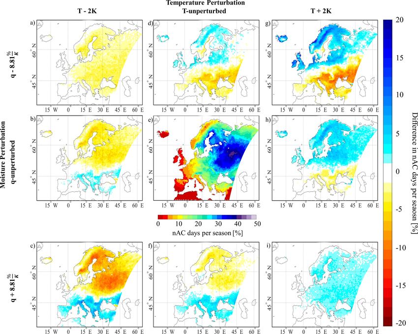
112 L. Jach et al.: Sensitivity of land–atmosphere coupling strength to changing atmospheric temperature
Table 1. Applied parameterizations of the simulations from Jach et al. (2020).
Model physics Parameterization scheme
Microphysics scheme New Thompson scheme (Thompson et al., 2004)
Shortwave radiation scheme Rapid Radiative Transfer Model (RRTMG) scheme (Iacono et al., 2008)
Longwave radiation scheme Rapid Radiative Transfer Model (RRTMG) scheme (Iacono et al., 2008; Mlawer et al., 1997)
Boundary layer scheme MYNN level 2.5 PBL (Nakanishi and Niino, 2009)
Convection scheme Kain–Fritsch scheme (Kain, 2004)
Land surface model Noah-MP land surface model (Niu et al., 2011)
Surface layer scheme MYNN surface layer scheme (Nakanishi and Niino, 2009)
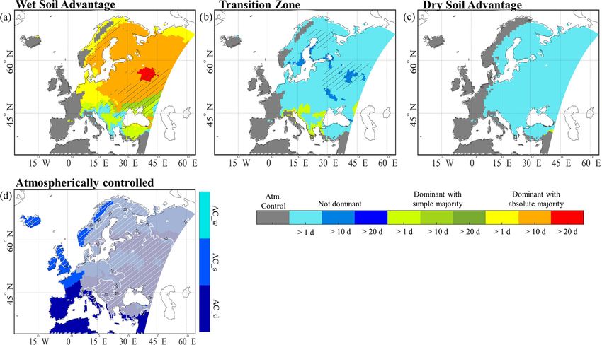
CTP and HIlow form the basis for categorizing early in the cell during the study period, while level-2 transition
morning ABL conditions on a daily basis in (1) prone-to- zone covers all cells remaining unlabeled.
triggering convection over wet or (2) dry soils, (3) a tran-
sition zone between wet and dry advantages, or (4) condi- 2.3 Modification approach
tions inhibiting a contribution of the land surface to the trig-
gering of deep convection. In the latter case, the occurrence Early morning profiles of temperature and moisture are re-
of precipitation is purely atmospherically controlled (AC). quired to compute the CTP-HIlow framework investigating
This can have three causes: either the ABL is very humid the pre-conditioning for convection triggering during the day.
(HIlow < 5 ◦ C) and rainfall is just as likely to occur over any Due to the large expansion of the domain covering several
surface, or the ABL is very dry (HIlow > 15 ◦ C) and moist time zones, the ABL evolution on the eastern edge of the do-
convection and precipitation rarely occur in general. Finally, main is in a different stage as that of the western edge at the
when the ABL is stable (CTP < 0 J kg−1 ), deep convection same UTC time step, which can lead to substantial differ-
is inhibited by an inversion. Only shallow clouds can oc- ences in the results of the coupling metric (Wakefield et al.,
cur. The first three defined classes (1–3) are jointly consid- 2021). Hence, the accurate UTC time step to depict the pre-
ered as non-atmospherically controlled (nAC). These indi- convective ABL for the coupling assessment cannot be uni-
cate the percentage of days within the study period with high fied throughout the domain. To ensure this comparability be-
potential for feedbacks of any kind. Triggering convection tween eastern and western Europe, we determined the sunrise
over wet soils (1) follows the hydrological pathway meaning hour in the model using shortwave downward radiation. The
positive soil moisture–evapotranspiration–precipitation feed- profiles were extracted for the UTC time step in which short-
backs. Hence, greater soil moisture leads to a moistening of wave downward radiation exceeded a value of zero the first
the ABL through evapotranspiration and more precipitation. time for each day and cell. The profiles from model output
Conversely, triggering convection over dry soils (2) occurs around local time sunrise of each day serve as the basis for
along the thermal triggering pathway during which a high the sensitivity analysis. In the following section, we describe
sensible heat flux leads to boundary layer growth and up- how the profiles were modified. The approach is based on our
ward mixing of moist air to heights where condensation and hypothesis that the temperature and moisture fields can vary
formation of rainfall can occur (Dirmeyer et al., 2014). In in terms of their mean, and their horizontal, vertical and tem-
the transition zone, convection can be triggered over wet or poral distributions. In this study, we investigate the impact of
dry soils, though no convection is the most likely outcome. modifying the mean and the vertical distribution. The tempo-
Here, we apply the original threshold values from Findell and ral and horizontal distributions were not modified, although,
Eltahir (2003a), which are shown in Fig. 1a. e.g., warming is known to widen and flatten the distribu-
The daily coupling classes are then used to derive a long- tion of temperature over time and therefore slightly change
term coupling regime for each grid cell, based on the relative the shape of the distribution. The processes and mechanisms
occurrence of each class during the study period (Fig. 1b). At leading to a change in the temporal distribution are complex
first, a cell with more than 90 % of the days in the study pe- and non-linear, meaning that they cannot be reproduced eas-
riod under atmospheric control is defined as AC. If this is not ily by the modifications. Differences in the spatial distribu-
the case, the partitioning of the nAC days in wet and dry soil tion (such as warmer conditions in France with colder con-
advantage, as well as transition zone days, is used to deter- ditions over eastern Europe) were not specifically depicted.
mine the dominant coupling class. A level-1 coupling regime The CTP-HIlow framework utilizes single columns and does
denotes that > 50 % of the nAC days in the cell are in the not recognize horizontal connections.
respective coupling class. Level-2 wet or dry soil advantage
means that less than 20 % of the respective other class occurs
Earth Syst. Dynam., 13, 109–132, 2022 https://doi.org/10.5194/esd-13-109-2022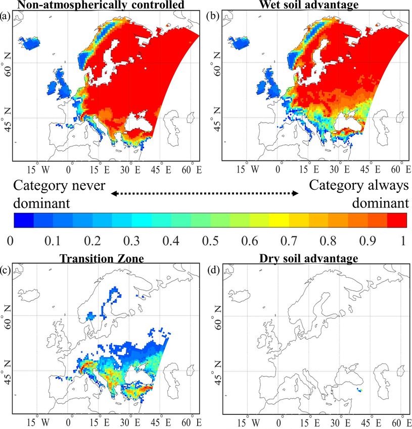
L. Jach et al.: Sensitivity of land–atmosphere coupling strength to changing atmospheric temperature                                      113

Figure 1. Schematic depicting the coupling strength classification with the convective triggering potential – low-level humidity (CTP-
HIlow ) framework by Findell and Eltahir (2003a, b) (adopted from Jach et al., 2020). Panel (a) shows the threshold values from Findell and
Eltahir (2003a); their Fig. 15. Panel (b) summarizes the approach for the long-term classification as explained in Findell and Eltahir (2003b).

2.3.1   Temperature modifications                                         midity, as well as (5) maximum near-surface specific humid-
                                                                          ity (wet_abs). The year with the minimum near-surface spe-
The temperature profiles were modified by adding a constant               cific humidity corresponds to the cold summer. Table 2 sum-
temperature (T ) factor in Kelvin to the daily profiles. The              marizes the years chosen for the divergence T factors and the
factor is fixed in time, homogeneous over the domain and de-              sign of their surface temperature and moisture anomalies, re-
creases with altitude. Decreasing the impact over height fol-             spectively. These were added to the temperature profiles from
lows the hypothesis that a surface temperature change does                the CTRL run on a daily basis. In a second step, the diver-
not propagate evenly throughout the atmospheric column.                   gence cases were further modified by adding the same factor
The T factor for each atmospheric layer was derived using a               used for the core set in order to investigate the effect of dif-
simple linear regression model and calculating the mean co-               ferences in the gradient with additional surface warming or
efficient of determination for each atmospheric layer. There-             cooling on the coupling strength. Larger modification factors
fore, it corresponds to the fraction of variance in temperature           up to ±5 K led to similar patterns of differences and diverged
for each atmospheric layer explainable by the temperature                 in the magnitude of the impact in most cases.
variance at the surface.
   The first set of temperature modifications (hereafter called
                                                                          2.3.2    Moisture modifications
the core set) captures differences in the mean air temperature
near the surface and in the vertical by applying the temper-              Besides the temperature, also the moisture content in the
ature factor. In this case, the modification amounts to ±2 K              atmosphere is expected to have an impact on the coupling
at the surface (= 2 × T factor). This range was derived from              strength. Willett et al. (2010) investigated the scaling of
the acceptable range of biases in temperatures in Kotlarski et            concurrent temperature and moisture changes for different
al. (2014). Plots with stronger modifications of ±5 K cover-              regions around the globe based on observations and mod-
ing the full range of the model bias of this particular run are           els. For the Northern Hemisphere, they found that tempera-
provided in the Supplement. A second set of modifications                 ture and moisture are strongly positively correlated and that
served to investigate the effect of differences in the shape of           1 K temperature changes corresponds to on average 8.81 %
the profiles (e.g., greater or smaller inversions) leading to dif-        change in moisture. The factors for northern (9.66 % K−1 )
ferences in the gradients. For this purpose, we determined the            and southern (7.74 % K−1 ) Europe slightly deviate. Under
divergence of the mean temperature profiles of summers with               the assumption that the scaling is valid through the entire at-
the highest near-surface temperature or near-surface moisture             mospheric column, the Northern Hemisphere factor was used
anomalies from the mean temperature profile of all 30 years               for the moisture modifications. Hence, the magnitude of the
to produce five divergence T factors. Chosen were the sum-                change is dependent on the respective temperature modifica-
mers with (1) minimum (cold) and (2) maximum (hot) near-                  tion and the moisture present in the atmosphere in the CTRL.
surface temperature, as well as the summers with the (3) min-             This ensures two things: first, the relation of temperature and
imum (dry) and (4) maximum (wet) near-surface relative hu-                moisture is maintained, and second, the higher atmospheric

https://doi.org/10.5194/esd-13-109-2022                                                        Earth Syst. Dynam., 13, 109–132, 2022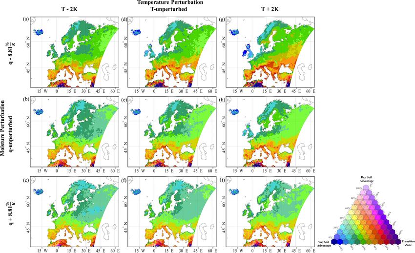
114                       L. Jach et al.: Sensitivity of land–atmosphere coupling strength to changing atmospheric temperature

Table 2. Anomalies from the JJA mean of the CTRL run in temperature and moisture in years chosen as basis for the alternative factors; ∗
indicates that the cold and dry_abs are the same year.

                                                                  Negative T anomaly                    Positive T anomaly
                                  Negative q anomaly          cold/dry_abs∗         dry             –           –          –
                                                              (1986)                (1994)
                                  Positive q anomaly          –                     –               hot         wet_abs    wet
                                                                                                    (2003)      (2010)     (2013)

layers do not experience unrealistic increases in moisture,                             ture control. With a sensitivity index around 0, moisture and
which could have occurred using fixed factors. As for the                               temperature variations have an equal impact on changes in x.
temperature modifications, the mean moisture and the shape                                 In this study, we used the temperature modification of
of the profiles were modified but the temporal and spatial                              ±2 K, and the cases with the corresponding moisture modifi-
variances were not.                                                                     cations of ±2·8.81 % K−1 , from the core modifications set to
   To further prevent the development of unrealistically high                           estimate the relative importance of temperature versus mois-
moisture content in the atmosphere in humid regions, the                                ture changes for CTP, HIlow and the occurrence of nAC days,
saturation vapor pressure was determined for the tempera-                               wet and dry soil advantage as well as transition zone days.
ture after modification and used to cap the moisture increase.                          We limited the analysis to regions where on average at least
Negative moisture content was prevented by setting a lower                              2 d per summer (∼ 2.5 % of the summer days) are in the re-
boundary of 0 g kg−1 . Thus, the relative humidity (in terms                            spective category.
of specific humidity divided by saturation specific humidity)
is designed to remain between 0 % and 100 % in all atmo-                                2.5    Uncertainty of hotspot location and feedback sign
spheric layers.
                                                                                        Two measures were used to depict the sensitivity of the
                                                                                        long-term coupling regimes in the modification cases. The
2.4    Statistical sensitivity assessment
                                                                                        first metric Ifeed measures the degree of agreement of the
A sensitivity index was used to achieve a grid wise estimate                            long-term classification based on the CTP-HIlow framework
whether temperature modifications or moisture modifications                             among the modification cases with that of the CTRL case.
have a higher impact on the corresponding variable. The in-                             A value close to 1 indicates that nearly all modifications had
dex compares the magnitude of differences in a variable x                               the same long-term coupling regime no matter which modi-
caused by modifying moisture or temperature only from the                               fication factors were applied. A value close to 0 indicates an
CTRL. The approach is described using the following for-                                overall disagreement in the long-term coupling regimes with
mula:                                                                                   the CTRL case indicating that the classification is sensitive
                                                                                        to differences in the temperature and moisture profiles.
xsens =
P                2             2  P              2             2                                n
                                                                                                        P
      xQlow − xref + xQhi − xref     −    xTlow − xref + xThi − xref                                        (catn 6 = catCTRL )
P                2             2  P              2             2  ,                             1
      xQlow − xref + xQhi − xref     +    xTlow − xref + xThi − xref                    Ifeed = 1 −                               ,                 (3)
                                                                                                                    n
                                                                              (2)
                                                                                               n
                                                                                               P
                                                                                        with       (catn 6 = catCTRL ) denoting the sum of modification
where xref is the value of the unmodified case, xQlow is the                                   1
value of the modification case of isolated decrease in mois-                            cases in which the long-term coupling regimes disagree with
ture, xQhi is the case with an isolated increase in moisture,                           that of the CTRL case, and n being the number of all modifi-
xTlow is the case with an isolated decrease in temperature, and                         cation cases tested. A second metric Icat was used to quantify
xThi is the case with an isolated increase in temperature, re-                          the share of modification cases in which each of the cou-
spectively. Thus, the modification cases with isolated temper-                          pling classes occurred. It was determined for nAC days, and
ature or moisture modifications were used for this analysis.                            days in wet soil advantage, dry soil advantage or transition
The index was then normalized to a value between −1 and 1                               zone. Level-1 and level-2 cells of the coupling classes were
by dividing the squared sum of differences induced by mois-                             grouped together before deriving the metric.
ture changes minus the squared sum of differences induced                                       P
                                                                                                   ncat
by temperature changes by the total squared sum of differ-                              Icat =          ,                                          (4)
ences from the CTRL in all cases. A sensitivity index close                                       n
to −1 indicates a strong temperature control on the variable,                           with ncat being the number of modification cases in the re-
while a sensitivity index close to 1 indicates a strong mois-                           spective regime. A value of 0 denotes that the class was never

Earth Syst. Dynam., 13, 109–132, 2022                                                                          https://doi.org/10.5194/esd-13-109-2022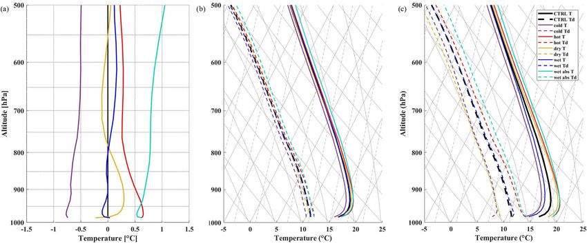
L. Jach et al.: Sensitivity of land–atmosphere coupling strength to changing atmospheric temperature                         115

dominant and a value of 1 denotes that the class was always         3.2     Sensitivity analysis
dominant.
                                                                    In this section, we describe how differences in the mean tem-
                                                                    perature and moisture profiles impact the frequency of favor-
3     Results                                                       able conditions for local land-surface-triggered deep convec-
                                                                    tion, how the likelihood for convection triggered over wet
3.1    Comparison model and reanalysis
                                                                    versus dry soils changes and how these influences are repre-
This section provides a statistical comparison of the mean          sented in classifications of long-term coupling regimes with
and temporal distribution of near-surface temperature and           the CTP-HIlow framework.
specific humidity from the CTRL run with an ERA5-based
bias-corrected reanalysis dataset (C3S, 2020) to quantify un-
certainty originating from climatological inconsistencies of        3.2.1    Regional differences introduced by modifications
the model as compared to the reanalysis data. The statisti-         In the core set, the modifications reach to approximately
cal analyses comprise of the bias and two measures to com-          500 hPa a.g.l. The cases cover a range of different combina-
pare the temporal distributions: a statistical z test and the       tions of temperature and moisture modifications to estimate
probability density function (PDF) skill score after Perkins        (1) modifications with the same sign that represent changes
et al. (2007).                                                      following the observed positive correlations between T and q
   The model has a dry bias over the Mediterranean, France          in Europe. Additionally, examining (2) the isolated effects of
and the British Isles, and the z test showed that the tem-          temperature and moisture allows for the disentanglement of
perature distribution is shifted towards warmer conditions          their impacts on the coupling strength as well as (3) modifi-
(Fig. 2a and b). Over the eastern part of the domain, the           cations with opposing signs. The core set aimed at covering
model has a cold bias and overestimates the frequency of            four possible combinations of differences in the climate con-
cooler days. The z value, which remained consistently be-           ditions, namely, cooler and moister conditions, cooler and
low 2 throughout the domain, indicated that the differences         dryer conditions, warmer and moister conditions, as well as
in the temporal distribution are statistically insignificant. The   warmer and dryer conditions.
PDF skill score drew a similar picture (Fig. 2c). The distribu-        Previous observational and global model studies suggested
tions strongly resemble with values > 0.8 over most of cen-         that temperature and moisture are considerably positively
tral and eastern Europe as well as over the high latitudes.         correlated in most regions around the globe and trends lie
The skill is weaker in the southern part of the domain. The         around 7 % change in moisture per Kelvin change in tem-
model particularly misrepresents the temperature distribution       perature, reflecting the Clausius–Clapeyron rate for increases
over the Alpine region, in the south of the Black Sea and the       in moisture, which maintains a quasi-constant relative hu-
northern African desert.                                            midity (Bastin et al., 2019; Willett et al., 2010). In Europe,
   The moisture bias is presented in terms of the specific hu-      the scaling of moisture to temperature was slightly higher
midity. The model has a dry bias of up to −2 g kg−1 over            (Sect. 2.3.2). In addition to the rates described before, a
the Mediterranean and southeastern Europe (Fig. 2d), which          rate of 5 % K−1 was tested to represent a change in mois-
corresponds to maximally 20 % difference from the climato-          ture per Kelvin change in temperature below the Clausius–
logical mean of the reanalysis data in summer. The specific         Clapeyron rate. Figure 3 depicts the divergence in frequency
humidity is slightly overestimated by up to 0.5 g kg−1 over         of nAC days from the CTRL run with 2 K warmer and
Scandinavia and the British Isles and slightly underestimated       cooler conditions for all land points. Impacts on the coupling
in central and eastern Europe in the same range. The dif-           strength and the pre-conditioning for the different coupling
ferences in specific humidity correspond to less than 10 %          regimes have the same sign for each tested rate. A higher
difference from the climatological mean (not shown). The            scaling of moisture with temperature – as observed in north-
z statistic showed that the temporal distribution of specific       ern Europe – enhanced the effects on the coupling.
humidity was shifted to dryer or more humid conditions cor-            For the following analysis, we combined the rate of the
respondingly (Fig. 2e). However, the z value remained con-          Northern Hemisphere (8.81 % K−1 ) with 2 K temperature
sistently below 1, indicating that the differences in the tem-      changes at the land surface. Figure 4 shows the coefficient of
poral distributions between model and reanalysis data are in-       determination used as basis for the modification over height
significant. Again, the PDF skill score matched the findings        as well as the temperature and dew-point temperature profiles
from the z statistic (Fig. 2e and f). The skill of the model        after modification. CTP and HIlow changes were uniform
to represent the distribution of specific humidity is partic-       throughout the domain. Their spatial patterns were largely
ularly high over the East European Plain and central Europe         maintained from the CTRL run, which were considered rea-
with scores mostly > 0.9. The skill is lower over the Mediter-      sonable (Jach et al., 2020). When temperature and moisture
ranean, dropping to a range between 0.4–0.6.                        modifications had the same sign (e.g., warmer and moister),
                                                                    the sign of differences in nAC days was uniform throughout
                                                                    the domain (Fig. 5a and i). Cooler and dryer conditions re-

https://doi.org/10.5194/esd-13-109-2022                                                  Earth Syst. Dynam., 13, 109–132, 2022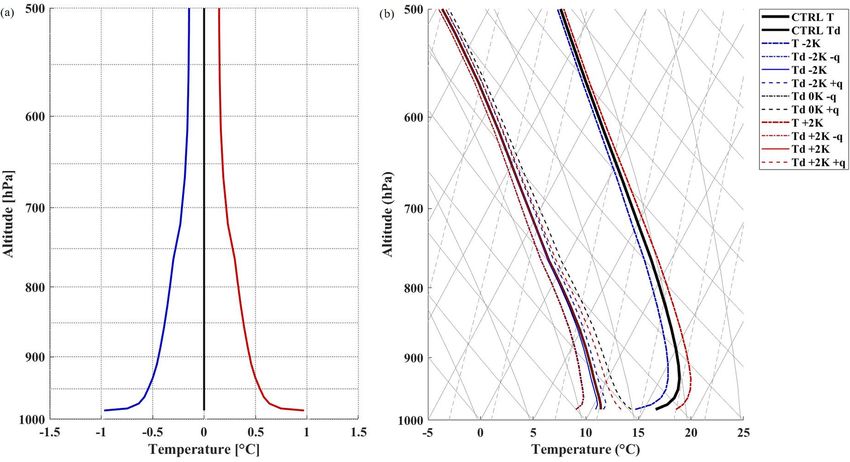
116                  L. Jach et al.: Sensitivity of land–atmosphere coupling strength to changing atmospheric temperature

Figure 2. Statistical metrics for comparison of modeled temperature and specific humidity from CTRL with bias-corrected ERA5 reanalysis
data (C3S, 2020). Panel (a) shows the value of a Z statistic comparing the temporal distribution of modeled temperature with reanalysis;
panel (b) shows the PDF skill score as a second measure to compare the temporal distribution of modeled temperature with reanalysis.
Panels (c, d) are the same as (a, b) but for specific humidity.

duced potential coupling days by about 5 %, whereas warmer            quence of more early morning profiles showing stable con-
and moister conditions increased the frequency of nAC days            ditions. Conversely, a warming initiated a strengthening of
by 3 %–5 %.                                                           the coupling (Fig. 5h). The impact was smaller in southern
   Analyzing the cases with individual modifications in tem-          Europe, and it switched sign. Lower temperatures reduced
perature and moisture was used to disentangle their respec-           the humidity deficit, and thus decreased the amount of days
tive impacts on different coupling variables. Isolated temper-        during which a low atmospheric moisture content inhibited
ature changes primarily influenced the coupling strength in           convective precipitation. Moisture modifications had a larger
northern Europe, where lower temperatures weaken the cou-             impact in the south of the domain. While dryer conditions
pling over energy-limited regions – such as Scandinavia and           were favorable for the occurrence of coupling days in the
over the East European Plain. This happened as a conse-               north, moister conditions were favorable in the south. The

Earth Syst. Dynam., 13, 109–132, 2022                                                     https://doi.org/10.5194/esd-13-109-2022
L. Jach et al.: Sensitivity of land–atmosphere coupling strength to changing atmospheric temperature                                   117

Figure 3. Changes in frequency of non-atmospherically controlled (nAC) days in response to different combinations of temperature and
moisture changes in the core modification set. m2K denotes a cooling by 2 K at the surface, p2K a warming of 2 K at the surface, m2per
denotes a drying of 2 times the scaling factor, and p2per denotes a moistening of 2 times the respective scaling factor in the domain for
different T − q scaling factors. Blue: 5 % K−1 , orange: 7.74 % K−1 , yellow: 8.81 % K−1 , purple: 9.66 % K−1 .

Figure 4. Temperature modification factor derived using a simple linear regression model and extracting the coefficient of determination
for each atmospheric layer (a). Profiles of temperature (T ) and dew-point temperature (Td ) after modification (b). Red indicates warmer
temperature and blue cooler temperatures, and unchanged temperature is denoted in black. Dash-dotted lines indicate a reduction in moisture,
solid lines unchanged moisture and dashed lines an increase in moisture.

same spatial patterns occurred when the implemented modi-               of the transition zone around the Black Sea remained unaf-
fications differed in sign (Fig. 5c and g). Spatial patterns of         fected. The spatial patterns of changes in wet soil advantage
impacts on the coupling variables were similar, and therefore           days closely followed that in nAC days in most modification
differences added up, leading to relatively high differences            cases. A change in the partitioning predominantly occurred
in the frequency of nAC days (Fig. 5c and g) and their par-             between wet soil advantage and transition zone days. Dryer
titioning in wet and dry advantages (Fig. 6). Differences in            and warmer conditions increased the frequency of transi-
the frequency of nAC days reached up to 10 % of the sum-                tion zone days relative to the CTRL case, vice versa for
mer days. Nevertheless, following the argument that mois-               moister and cooler conditions. Any modification case initi-
ture scales positively with temperature, real-world tempera-            ated a dominant dry soil advantage.
ture and moisture impacts are expected to counteract each                   The impact on the long-term classification of coupling
other, leading to weak net effects.                                     regimes did not reflect the changes in nAC days and their par-
    The partitioning of nAC days experienced some small                 titioning in wet and dry advantages for convection (Fig. 7).
shifts of up to ±10 % between the categories (Fig. 6). The              Differences to the CTRL case mainly occurred over eastern
predominance of the wet soil advantage in the north and                 Europe at the edges of the coupling region, and the predomi-

https://doi.org/10.5194/esd-13-109-2022                                                      Earth Syst. Dynam., 13, 109–132, 2022
118                   L. Jach et al.: Sensitivity of land–atmosphere coupling strength to changing atmospheric temperature

Figure 5. Difference in the seasonal share of non-atmospherically controlled (nAC) days [%] from CTRL for each modification case of the
core set. The center image is the CTRL case modified after Jach et al. (2020) (their Fig. 4g). The columns denote the temperature change and
the rows the relative change in moisture.

nance for positive feedbacks remained unchanged also in the             dex of −1 throughout the domain (not shown). In the case
cases with strong changes in relative humidity. The modifi-             of HIlow , the impacts of temperature and moisture modifi-
cations initiated changes between wet soil advantage levels 1           cations were of similar magnitude, though, moisture had a
and 2, as well as transition zone levels 1 and 2. None of the           slightly higher impact, indicated by small but positive val-
modification cases experienced a considerable shift in loca-            ues. The magnitude of temperature and moisture controls on
tion or a change in the predominant sign of feedbacks com-              HIlow became more equal in mountainous regions.
pared to the CTRL (Figs. 6 and 7).                                         The sensitivity index for the share of nAC days in sum-
                                                                        mer showed a clear dipole pattern (Fig. 8a). In northern Eu-
3.2.2   Sensitivity of the coupling to separated changes in             rope, the coupling is rather impacted by temperature varia-
        temperature and moisture                                        tions. Temperature controls the coupling by determining the
                                                                        stability of the atmosphere.
This section further examines the relative importance of tem-              In southern Europe, moisture was the controlling factor,
perature versus moisture modifications for the variables CTP,           and little relative humidity in the low-level ABL limits the
HIlow , as well as the share of nAC days, wet soil advantage,           occurrence of feedbacks in consequence of limited mois-
transition zone and dry soil advantage days in Europe. The              ture availability for deep moist convection. The sensitivity
sensitivity index as described in Sect. 2.4 was used to esti-           index computed for the wet soil advantage showed a sim-
mate the magnitude of the control of temperature and mois-              ilar pattern. Hence, sensitivity of the coupling exhibited a
ture relative to each other for each variable throughout the            regional dependency to temperature and moisture changes,
domain.                                                                 which hints at humidity- and energy-limited regimes con-
   The temperature and moisture modifications changed CTP               trolling the coupling. The dry soil advantage rarely occurred,
and HIlow linearly. Differences in CTP, the stability of the at-        but its occurrence is rather controlled by temperature vari-
mospheric layering, were almost solely controlled by modi-              ations in northeastern Europe (Fig. 8d) and by moisture in
fications of the temperature, as indicated by a sensitivity in-

Earth Syst. Dynam., 13, 109–132, 2022                                                       https://doi.org/10.5194/esd-13-109-2022
L. Jach et al.: Sensitivity of land–atmosphere coupling strength to changing atmospheric temperature 119
Figure 6. Composition of the non-atmospherically controlled days comprising wet soil advantage, dry soil advantage and transition zone
days for all core modification cases. The columns denote the temperature change and the rows the relative change in moisture.
southeastern Europe. The sensitivity of the transition zone with an increase in moisture (thus a moistening) of the ABL
shows a complete different pattern. The moisture modifica- with positive temperature–moisture relationship. As CTP is
tions caused higher differences in the occurrence of transi- almost entirely controlled by the air temperature, this prac-
tion zone days in the coupling hotspot, while temperature tice only affected HIlow .
modifications only had a higher impact towards the south- We first investigated the impact of shifting the tempera-
west (Fig. 8c). ture and moisture gradients from the CTRL case using the
divergence factors of the extreme years (see Sect. 2.3.1). The
3.2.3 Effects of changing temperature and moisture
main impact concerned changes in CTP, since this is an inte-
gradients
grated variable. Changes in the temperature gradient moved
the lapse rate more toward the dry or moist adiabats, and
The following section deals with the analysis of how changes hence influence the atmospheric stability. The hot and the
to steeper or less steep temperature and moisture gradients dry divergence factors increased the early morning tempera-
can influence the coupling classification and to compare how ture gradients between 100–300 hPa above ground, shifting
such differences can impact the result of the coupling metric. them closer to the dry adiabat, but also enhanced the sur-
Figure 9 shows the divergence factors for each case which face inversion (Fig. 9). This caused an increase in CTP, while
were derived from the temperature difference of the corre- the enhancement of the surface inversion, which is likely re-
sponding summer (Table 2) from the climatological mean sulting in a higher convective inhibition, is not accounted
temperature averaged over the domain. The other subplots for in the framework. In the other three cases (cold, wet,
show the resulting temperature and dew-point temperature wet_abs), the temperature gradient was decreased between
profiles in the lower ABL. For the cases chosen because of 100–300 hPa a.g.l., consequently decreasing CTP (Fig. 10).
their moisture anomaly – namely the dry and the wet cases The cases diverge in the mean temperature change among
– the moisture factor was derived by multiplying the T fac- each other. Likewise, the temperature inversion decreased in
tor with −1 to derive moister conditions in the wet and dryer the lower atmospheric layers (Fig. 9). Differences in HIlow
conditions in the dry case. This was done to circumvent that, resulted from both temperature and moisture changes. How-
in the dry case, a higher temperature would be associated ever, HIlow changes were small in most cases (Fig. 10),
https://doi.org/10.5194/esd-13-109-2022 Earth Syst. Dynam., 13, 109–132, 2022120 L. Jach et al.: Sensitivity of land–atmosphere coupling strength to changing atmospheric temperature
Figure 7. Long-term classification of coupling regimes for the core set modification cases. The columns denote a temperature change and
the rows a change in moisture. The center image is the CTRL case and modified after Jach et al. (2020) (their Fig. 3a). The columns denote
the temperature change and the rows the relative change in moisture.
because temperature and moisture change simultaneously, creased the expansion of the hotspot and the fraction of
which led to small changes in relative humidity. The only nAC days within the L–A coupling hotspot.
considerable exception was the dry case, where the T factor
was multiplied by −1. In this case, HIlow increased by about – The dry case involved a larger temperature gradient but
1 ◦ C. less moisture in the atmosphere. A greater instability
The combination of temperature and moisture changes in was combined with a higher humidity deficit, which
each case determines the difference for the share of nAC jointly caused an increase in the fraction of nAC days
days (Fig. 11a). The effects are summarized in the follow- in summer in the hotspot, but the area of the domain in-
ing points: cluded in the hotspot remained unchanged. Higher hu-
midity deficits reduced the coupling of land surface and
convection around the Black Sea but increased the like-
– In the hot case, a higher temperature and temperature lihood for convection triggering over wet soils in the
gradient between 100–300 hPa a.g.l. was caused with north.
corresponding changes in moisture. These led to greater
instability with a constant humidity deficit, which in-
Earth Syst. Dynam., 13, 109–132, 2022 https://doi.org/10.5194/esd-13-109-2022L. Jach et al.: Sensitivity of land–atmosphere coupling strength to changing atmospheric temperature 121
Figure 8. Sensitivity score of (a) non-atmospherically controlled days per summer season, (b) wet soil advantage days per summer season,
(c) transition zone days per summer season and (d) dry soil advantage days per summer season to changes individual modifications in the air
temperature profile (−1 indicates totally temperature controlled) and specific humidity profiles (1 indicates totally humidity controlled).
– The cold case resulted in a combination of lower tem- sion of the transition-zone-labeled region over land. Though
perature, a decrease in the temperature gradient between the dry soil advantage never became dominant, which can be
100–300 hPa a.g.l. and moisture changes corresponding seen in the unchanged expansion over land (Fig. 11d), tem-
to 8.81 % K−1 , which led to a reduction in the expan- perature changes still influenced the frequency of days dur-
sion of the hotspot region in the study area and a loss of ing which negative feedbacks could occur. Similar to the wet
nAC days. soil advantage, higher temperatures increased the frequency
of days in dry soil advantage during summer.
– The wet_abs and wet cases showed temperature in-
creases but shallower temperature gradients with corre-
sponding changes in moisture, which resulted in minor 3.3 Uncertainty of the coupling regimes
impacts on the coupling.
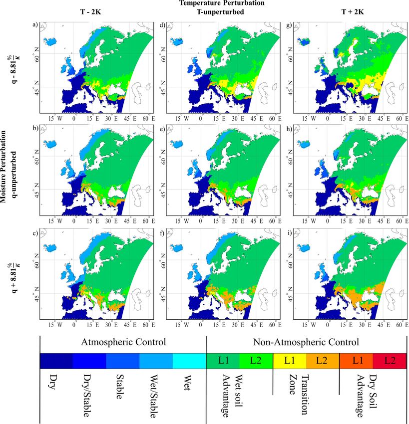
Here, we examine changes in the occurrence of the coupling
Further examination of the differences in the share of the classes during summer which is based on the daily classifica-
coupling categories shows that the area in wet soil advantage tion (comp. Fig. 1a), and to which extent the long-term clas-
shrinks in all divergence cases (Fig. 11b). Warmer tempera- sification, indicating the dominance of a coupling class in a
tures strengthened the frequency of the wet soil advantage in cell, reflects these changes. Under the assumption that the
the hotspot and cooling weakened it. Days in the transition modification cases cover a reasonable spread in atmospheric
zone experienced the opposite effect (Fig. 11c). However, all temperature and moisture for the prevailing climate, it aims
combinations of changes in the gradients led to an expan- at understanding how sensitively the coupling strength and
https://doi.org/10.5194/esd-13-109-2022 Earth Syst. Dynam., 13, 109–132, 2022122 L. Jach et al.: Sensitivity of land–atmosphere coupling strength to changing atmospheric temperature
Figure 9. (a) Divergence temperature (T ) factors derived from differences of the domain average temperature profiles of the corresponding
summers to the 30-year mean (Table 2) which were used to modify daily model output, (b) domain average of T and Td profiles for the
divergence T factors, and (c) their additional modifications with the core T factor. Purple: cold, red: hot, yellow: dry, blue: wet, turquoise:
wet abs; solid lines represent temperature and dashed lines represent dew-point temperature.
occurrence of each coupling regime in the modification cases
using Eq. (4) to explore which coupling regimes occurred in
the different cases. The Iberian Peninsula, northern Africa
and the northeast of Europe showed high agreement in the
regime classification of all modification cases and thus low
sensitivity to temperature and moisture changes. Over the
Iberian Peninsula and over northern Africa, the dry atmo-
spheric controlled regime reliably predominated in all cases,
whereas over northeastern Europe, it was reliably classified
in one of the nAC coupling regimes (Fig. 13a). In the transi-
tion between these two regions there was a belt, where the
coupling regime changed on a regular basis. Thus, it ap-
peared to be sensitive to temperature and moisture changes.
The absence of several coupling regimes suggests that over
Scandinavia, the British Isles and central Europe, the ques-
tion is whether or not feedbacks occur. When feedbacks oc-
Figure 10. Changes in convective triggering potential (CTP) and
curred, wet soils were in favor (Fig. 13a and b). In southeast-
low-level humidity index (HIlow ) due to the divergence factors.
ern Europe, from the Alps to around the Black Sea, summers
were reliably in non-atmospherical control (Fig. 13a), but the
dominant coupling regime switched between wet soil advan-
the pre-dominant coupling class respond to temperature and tage and transition zone (Fig. 13b and c). Some cells had an
moisture differences within this spread. For this purpose, we equal share of modification cases in wet soil advantage and
first looked at the sensitivity of the long-term regime clas- transition zone. A dominant dry soil advantage occurred only
sification by determining the share of modification cases in in single cells and cases over Turkey.
which the coupling classification coincided with that of the Secondly, we explored differences regarding the occur-
CTRL case (Fig. 12). A high share as assessed with Eq. (3) rence of the different coupling classes within all summer
indicated high agreement in the classified coupling regimes days between the modification cases. This is based on the
of the modification cases (red areas), and therefore low sensi- daily classification of the profiles in CTP-HIlow space. The
tivity, while green-to-blue colors indicate weak or no agree- analysis of sensitivity in the long-term coupling regimes al-
ment of the modified coupling regimes with that of the CTRL lows to distinguish five regions used for a spatial aggrega-
case and therefore high sensitivity. Please note that no agree- tion: (1) pure nAC, where less than two modification cases
ment also involves changes between a coupling regime in changed the coupling regime maintaining nAC in nearly
level 1 and level 2. We further quantified the frequency of
Earth Syst. Dynam., 13, 109–132, 2022 https://doi.org/10.5194/esd-13-109-2022L. Jach et al.: Sensitivity of land–atmosphere coupling strength to changing atmospheric temperature 123
Figure 11. Impacts of the divergence cases on the spatial expansion and the occurrence of the coupling classes in summer for (a) non-
atmospherically controlled (nAC) days, (b) wet soil advantage (WSA), (c) transition zone (TZ) and (d) dry soil advantage (DSA). The x axis
depicts the changes in the average frequency of occurrence during summer and the y axis shows changes in the fraction of land area covered
by the respective coupling regime.
all cases, and (2) pure AC, where less than two modifica- In the pure AC region, the modification cases’ impact on
tion cases changed the coupling regime maintaining AC in the distribution was negligible. Dry AC days dominated, and
nearly all cases. Further, there are three regions with frequent modifications of temperature and moisture barely influenced
switches (at least two cases) in the coupling regime. In re- the atmospheric pre-conditioning. Considerable variance in
gion (3), the coupling regime changed between any AC class the occurrence of coupling days of in part more than 20 %
and the wet soil advantage, in region (4) the changes were of the summer days occurred mainly in the hotspot region
between AC classes, the wet soil advantage and the transi- (Figs. 14 and 15d). In the pure nAC region, the number of
tion zone, and in region (5) the changes were between the nAC days ranged on spatial average between 19.2 and 28.5 d
wet soil advantage and the transition zone. The cell remained per season. The number of wet soil advantage days was rela-
in nAC in any of the modification cases. Figure 14 shows tively stable (ranged between 12.4 and 17.7 d), but the num-
the distribution of summer days in the coupling classes for ber of transition zone days varied in part considerably (be-
these regions and all cases. Figure 15 further adds sensitiv- tween 4.3 and 11.8 d) with cases showing warming and great
ity maps depicting the average dominance of each coupling relative drying (p2K–m2per, dry amplification) having the
regime relative to the other coupling classes and their occur- most days in transition zone (Figs. 14a and 15b).
rence (given in days) in summer. Hatched areas denote that As indicated before, the classification was most variable
the number of days in the respective coupling regime varied in the WSA–TZ transition region. Similar to the pure nAC
considerably by more than 10 % of the summer days between region, the number of nAC days varied in spatial aver-
the modification cases. age between 15 and 26.1 d between the modification cases
(Fig. 15d), but in contrast to the pure nAC region, the num-
https://doi.org/10.5194/esd-13-109-2022 Earth Syst. Dynam., 13, 109–132, 2022You can also read